Non-Newtonian fluids
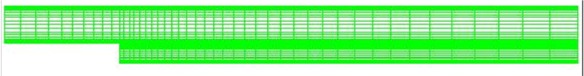
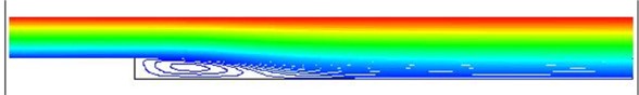
Turbulent flow over a backward facing step
Mesh
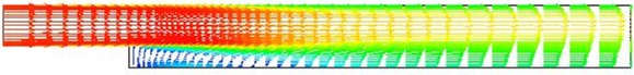
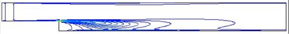
Steamlines
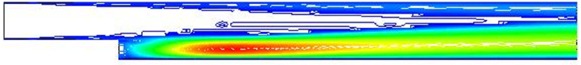
Velocity field
Turbulent kinetic energy (min=, max=)
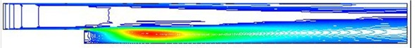
Turbulent dissipation rate (min=, max=)
Turbulent viscosity (min=0.0, max=0.01863)
Step height = 1, width before the step = 2, length before the step = 6
width after the step = 3, length after the step = 24 (has to be much longer than the recirculation length).
Inlet velocity = 1, fluid viscosity=2.2222e-5, Reynolds number based on the step heght and inlet velocity = 45,000
Summary
                            Recirculation length   % error         y+ value     # of iterations
                                   X_R

Experiment                     7.0+/-0.5

Standard k-epsilon                 6.5             -7.1           20 --> 610       83

Extended  k-epsilon, original      8.1             15.7           20 --> 573       39

Extended  k-epsilon, revised       6.6             -5.7           20 --> 598       41

RNG  k-epsilon (original)          7.4              5.7           20 --> 555       36

RNG  k-epsilon (revised)           7.3              4.3           20 --> 502       62
The recirculation length was obtained by plotting UX along a line with PVECTOR =(6.,-0.9,0.,1.,0.,0.), namely, on a line very close to the bottom boundary after the step.
My Gambit file for the above problem may be found here. My FIPREP file is attached here. Note that there is a problem of computing the yplus value at the bottom corner of the step.Modeling moving boundaries in FIDAP
What is ``The Moving-Body Constraint'' Capability?
How to provide a user subroutine?
FIDAP includes a capability which allows the user to define constraints that are applied and released as a function of time and position for the various nodal degrees of freedom. One application of such constraints is the modeling of a solid body moving through a continuum of fluid; therefore, the new capability is referred to as the "moving-body constraint" capability.
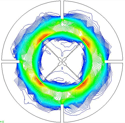
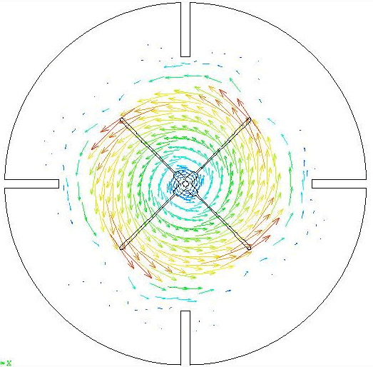
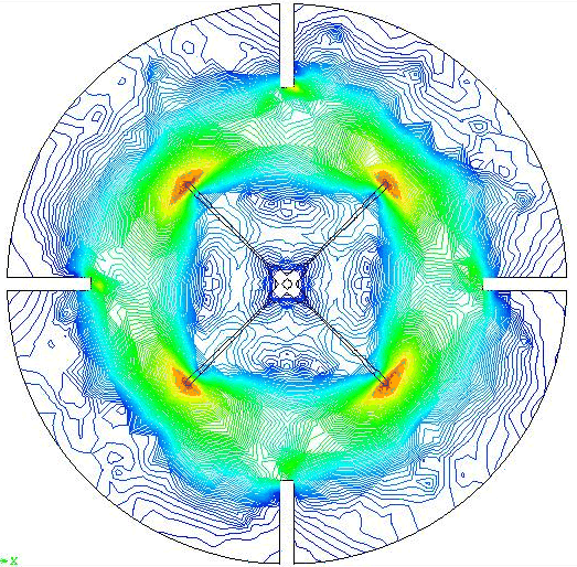
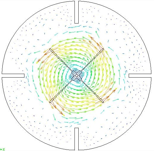
A typical application for the moving-body constraint capability is the modeling of a stirred, baffled tank such as that shown schematically in Figure 1, in which the velocity along the walls and baffles is zero, and the velocity along the blades is given by the rotational speed. At any given time step, the nodes associated with the blade may be given their appropriate boundary conditions or constraints. At the next time step, however, the blade is in a different position, therefore the previous constraints must be removed and new constraints applied. The moving-body constraint capability may be used in such instances to apply and remove constraints in a systematic fashion.
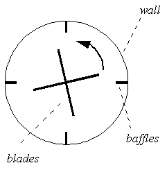
Figure 1
: Schematic of stirred tank with
baffles
In addition to constraints based on position, time and/or solution, any given nodal
degree of freedom (for example, temperature) may be constrained based on the value of
other degrees of freedom (for example, velocity). As a result, the moving-body capability
allows the construction of complex, solution-dependent nodal constraints which may be used
in either steady-state or transient simulations.
Problem Definition
Consider a mixing tank such as that shown in Figure 1 containing a fluid with the properties of water. The tank is 2 meters in diameter and includes four blades of radius 0.5 meters rotating at a speed of 1.047 rads/s (approximately 10 rpm). It also includes four baffles having a width of 0.3 and a thickness of 0.05 meters. The walls and baffles receive no-slip boundary conditions through the standard application of the BCNODE command. The moving blades are modeled using a moving-body constraint.
Figure 2 shows the two-dimensional mesh for the situation described above. The mesh is composed of two continuum entities: an "inner" entity, swept by the rotation of the blades, and an "outer" entity, completing the mesh. Only the inner entity is flagged as MOVING. At each time step, it is intended that the blades coincide with the nodal points of the mesh, therefore the mesh has a fan-type topology in the region swept by the blades. A fixed time step is used to ensure that the moving-body constraints are placed on element boundaries for each time step. (This approach is recommended but not required under the moving-body constraint.)
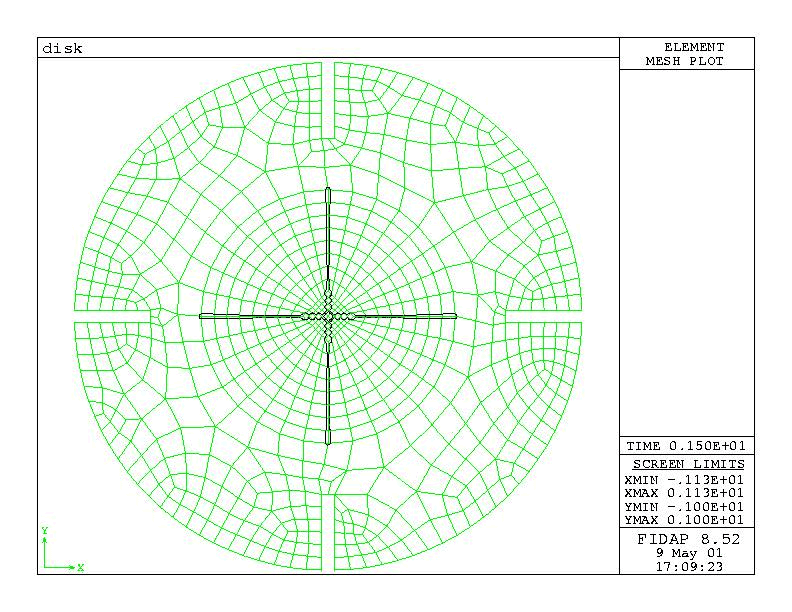
Figure 2a : Stirred Tank mesh
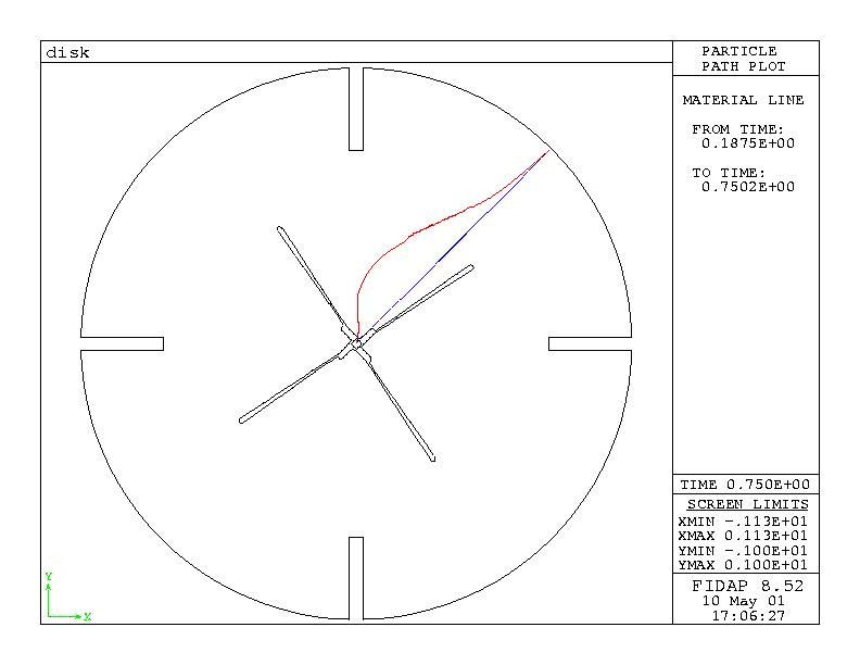
Figure 2b : Material trace
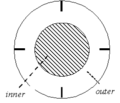
Figure 3 : Domain decomposition.
The mesh was generated by Gambit with the journal file given here.
The user subroutine USRMBC for this example is given here. At a given value of time, the four blades are located based upon their spatial (x ,y ) location. The variables XANG and YANG represent the intersection of the particular blade with the unit circle. The variables XV and YV represent the normalized coordinates of the node. The node is considered part of the blade if the normalized distance between (XV,YV ) and (XANG,YANG ) is less than a prescribed tolerance of 0.02. The velocity on the blades is defined as ,where is the rotation speed.
The FIPREP part of the problem setup is given here. The key points to note are the use of upwinding to address the convective nature of the flow equations and a fixed time step. The Reynolds number is about 13, based upon the blade tip speed.
The NOPREDICTION keyword is used in the TIMEINTEGRATION command, thus specifying that the solution from the time step be used as the prediction for time step . The predicted solution is actually further away from the corrected solution than is the previous solution. Absence of the NOPREDICTION keyword increases the number of nonlinear iterations required for each time step. The use of the NOPREDICTION keyword is generally recommended for transient moving-body constraint simulations.
Steps to include a User Subroutine:
Many of the advanced capabilities in FIDAP are accessed through user-supplied subroutines. In general, each user subroutine requires the computation of a given quantity -- for example, a fluid property or source term -- at a specified number of points. When the FIDAP solver module, FISOLV, operates in the scalar mode, these points typically represent integration points within a single finite element. When FISOLV operates in the vector mode, these points are integration points within a group of elements. The user subroutine is called only once for each element (or group of elements) in the computational mesh.
All of the FIDAP and FISOLV user-definable subroutines are available in two template files:
fidap_user.F -- FIDAP subroutine template file
fisolv_user.F -- FISOLV subroutine template file
In order to employ a user subroutine, you must edit its corresponding routine in the appropriate template file, then incorporate the template file into an executable version of the
FIDAP or FISOLV program. The procedures required to create executable versions of FIDAP or FISOLV that incorporate user subroutines depend on system type and vary
significantly from platform to platform. The FIDAP program package includes platform-independent utilities that isolate the user from system dependencies and simplify the procedure
for creating executable files.
(1) The get_fidap and get_fisolv utilities copy the fidap_user.F and fisolv_user.F template files, respectively , to your working directory.
(2) Modify the User subroutine.
(3) make_fidap user_routine.F creates an executable file named user_routine that incorporates user subroutines contained in the user_routine.F file. For example, the command
make_fidap fidap_user.F
creates an executable file named fidap_user .
make_fisolv user_routine .F creates the following two executable FISOLV files, each of which incorpo
rates user subroutines contained in the template file:
user_routine -- scalar version of FISOLV
user_routine _vec -- vector version of FISOLV
For example, the command
make_fisolv fisolv_user.F
creates two executable files, named fisolv_user and fisolv_user_vec.
(4) Load (or link) the compiled object user-subroutine template file with the provided library and object files for FIDAP (or FISOLV) to create the new executable.
fidap -id disk -new -gui -fidapexec fidap_user
fidap -id disk -new -gui -fisolvexec fisolv_user
Results
The results (velocity vectors and shear rate contours) at time step = 4 are shown here. The FILL (DISPLAY - FILL - species = 14 (IFLAG): Input = 1, value =0.9) command was used to outline the shape of the moving blade within the mesh. A contour value of 0.9 is chosen in order to keep the outline visually thin.
Bingham Plastic Fluid?
Modifications to the FIPREP file:
/ The fluid is Non-newtonian
 PROB (2-D, TRAN, NONL, NONN)
/ Newtonian viscosity = 0.02, yield stress = 0.04
 VISC (SET = 1, BING)
   0.2000000000E-01,  0.4000000000E-01
Results
The results (velocity vectors and shear rate contours) at time step = 4 are shown here.