MEEG 681 / MEEG481
Computer Solution of Engineering Problems
Computer Session 10
Outline and Objectives:
- Solve a dynamic (time-integration) problem in ANSYS
- Demonstrate nonlinear procedure and time integration
- Demonstrate time-history post processing in ANSYS
Different types of structural analyses in ANSYS (taken from ANSYS Structural Analysis Guide)
- 1. Static Analysis: A static analysis calculates the effects of steady loading conditions on a structure, while ignoring inertia and damping effects, such as those caused by time-varying loads. A static analysis can,
however, include steady inertia loads (such as gravity and rotational velocity), and time-varying loads that can be approximated as static equivalent loads (such as the static equivalent wind and
seismic loads commonly defined in many building codes).
- 2. Modal Analysis: modal analysis is used to determine the vibration characteristics
(natural frequencies and mode shapes) of a structure or a machine component while it is being designed.
It also can be a starting point for another, more detailed, dynamic analysis, such as
a transient dynamic analysis, a harmonic response analysis, or a spectrum analysis.
- 3. Harmonic Response Analysis: Any sustained cyclic load will produce a sustained cyclic response (a harmonic response)
in a structural system. Harmonic response analysis gives you the ability to predict the sustained dynamic
behavior of your structures, thus enabling you to verify whether or not your designs will successfully overcome
resonance, fatigue, and other harmful effects of forced vibrations.
- 4. Transient dynamic analysis (sometimes called time-history analysis): is used to determine the dynamic response of
a structure under the action of any general time-dependent loads. You can use this type of analysis to determine
the time-varying displacements, strains, stresses, and forces in a structure as it responds to any combination
of static, transient, and harmonic loads. The time scale of the loading is such that the inertia or damping effects
are considered to be important. If the inertia and damping effects are not important, you might be able to use a
static analysis instead.
- 5. Spectrum Analysis: A spectrum analysis is one in which the results of a modal analysis are used with
a known spectrum to calculate displacements and stresses in the model. It is mainly used in place of a time-history
analysis to determine the response of structures to random or time-dependent loading conditions such as earthquakes,
wind loads, ocean wave loads, jet engine thrust, rocket motor vibrations, and so on.
- 6. Buckling Analysis: Buckling analysis is a technique used to determine buckling loads - critical loads at which
a structure becomes unstable - and buckled mode shapes - the characteristic shape associated with a
structure's buckled response.
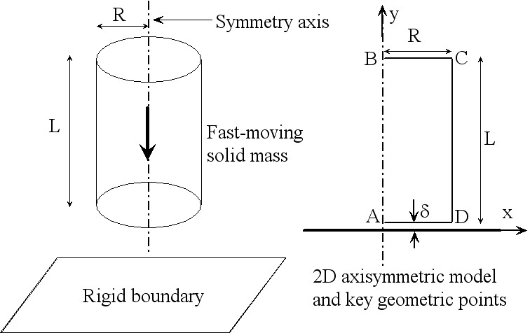
The transient problem: Aluminum Bar Impacting a Rigid Boundary

This problem is adapted from the ANSYS benchmark test problem C8.
A cylindrical aluminum bar impacts a rigid wall at a velocity Vo = 478 m/s. Determine the deformed length of the bar.
Key specifications:
- Cylinder radius = 0.381 cm, length = 2.347 cm.
- Density = 2700 kg/m3, Young's modulus = 70E9 Pa, Poisson Ratio = 0.3
- Bilinear isotropic hardening with yield stress at 420E6 Pa and tangential modulus at 100E6 Pa.
Solution Procedure and initial/boundary conditions:
- The edge AB (symmetry line) is assigned zero displacement in x direction for
all load steps.
- The solution was done by two load steps:
First load step: With low boundary at y = delta = 0.01 cm. Time step size =
0.0001/478 = 2.092E-7 s. So all nodes will be moved by a same distance of delta.
The low boundary AD was placed initially at y = delta.
The low boundary comes in contact with the rigid boundary at the end of
this first load step, all elements/nodes have an initial velocity of 478 m/s.
During the this load step, time integration (or solid mass inertia) was not
considered. The first load step sets up the proper initial condition!
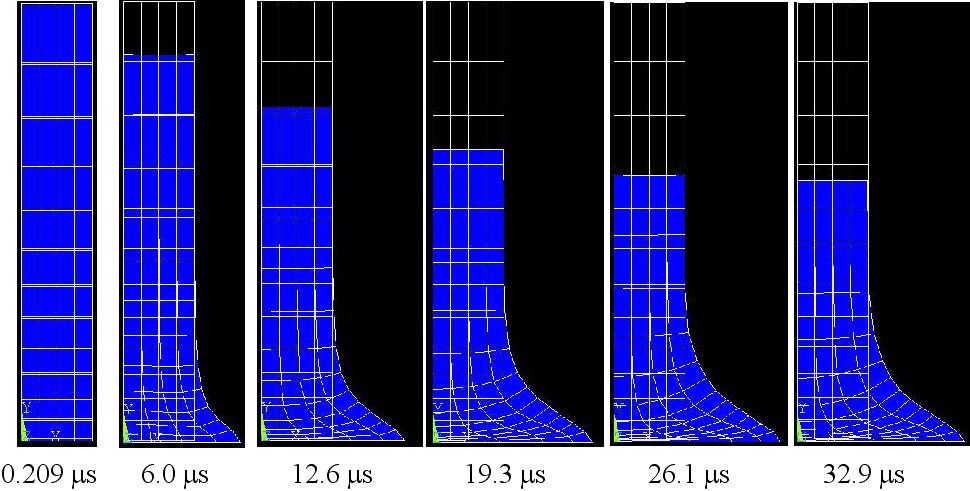
For the second load step, the transient (dynamic) evolution is considered.
The low boundary AD was held fixed at y = -delta (essentially zero). The time step size
was set according to the elastic wave propagation speed such that
the elastic wave cannot pass over more than one grid. The solution
was integrated until the displacement at the free end, point B,
is no longer changing. The total integration time was about 4.5E-5 s
and this took about 270 time steps. The transient solution is saved
every 10 substeps for time-history postprocessing and for time-dependent
visualization.
- Large deformation effects are included in the analysis.
- Use automatic time stepping and the Newton-Raphson method.
The original description of the problem is found here.
I performed an axisymmetric analysis with the
PLANE82 element.
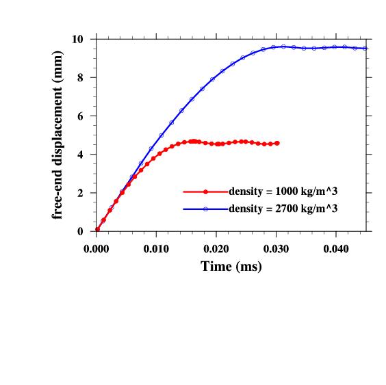
I tried two different material densities and compared the results below:
| Density |
Final Length (ANSYS) |
Final Length (Experiment) |
| 2700 kg/m3 |
1.405 cm (6.5% larger) |
1.319 cm |
| 1000 kg/m3 |
1.898 cm |
-- |
ANSYS log file with detailed set-up explanations:
impact-case1.input
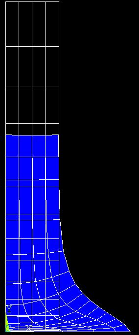
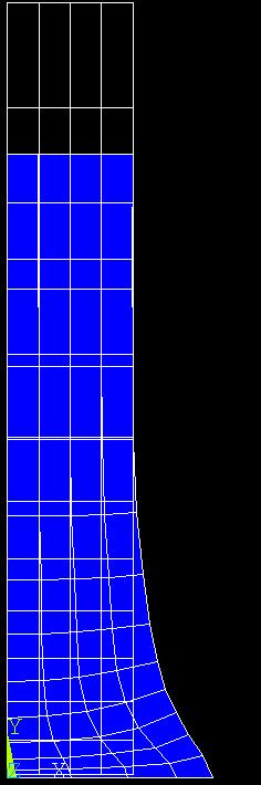
FINAL SHAPE. Left: density = 2700 kg/m3. Right density= 1000 kg/m^3. All other material properties
are the same.
Displacement at free end, point B.
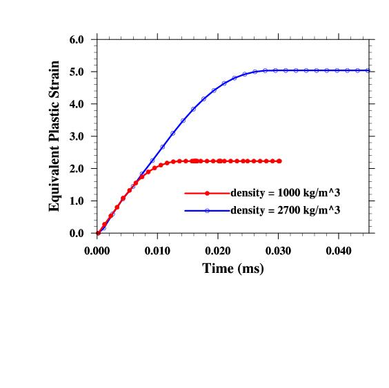
Equivalent plastic strain at point A.