
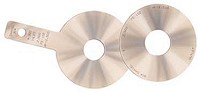
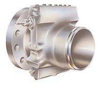
Orifice plates and fitting
Lecture: Tuesday, April 10, 9:30-10:45 in 007 Willard Hall
Lab Sessions: You need to attend one of the following lab sections:
Section 020, Tuesday, April 17, 12.30am-1.30am, 140 Dupont
Section 021, Tuesday, April 17, 5.00pm-6.00pm, 140 Dupont
Section 022, Tuesday, April 17, 6.00pm-7.00pm, 140 Dupont
Section 023, Thursday, April 19, 9.30am-10.30am, 140 Dupont
section 024, Thursday, April 19, 12.30am-1.30am, 140 Dupont
Section 025, Thursday, April 19, 5.00pm-6.00pm, 140 Dupont
Section 026, Thursday, April 19, 6.00pm-7.00pm, 140 Dupont
Objectives:
What is Gambit?
Gambit is a pre-processing software distributed by Fluent, Inc. to help create quickly geometry and high-quality mesh to be used by Fluent solver.
For further details, see GAMBIT webpage.
What is FLUENT?
FLUENT is distributed by Fluent Inc. and is a state-of-the-art computer program for modeling fluid flow and heat transfer in complex geometries. It contains an integrated set of components and program modules that allow fluid flow analysis for a wide variety of problems.
For further details, see FLUENT webpage.
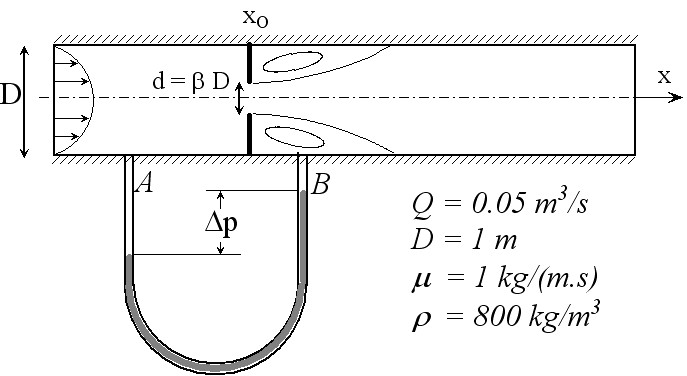
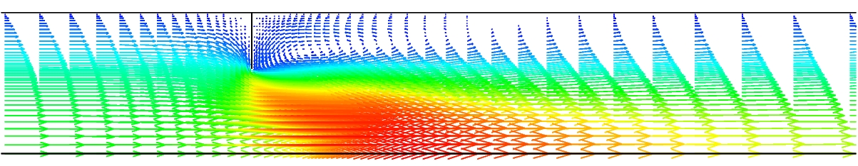
Flow modeling in a pipe with a concentric orifice plate
Orifice plates and fitting
1. Pipe diameter D = 1 m, fluid viscosity m = 1 kg/(m.s), density r = 800 kg/m3.
2. Orifice diameter d = 0.6D (model2)
3. Total in-coming flow rate Q = 0.05 m3/s
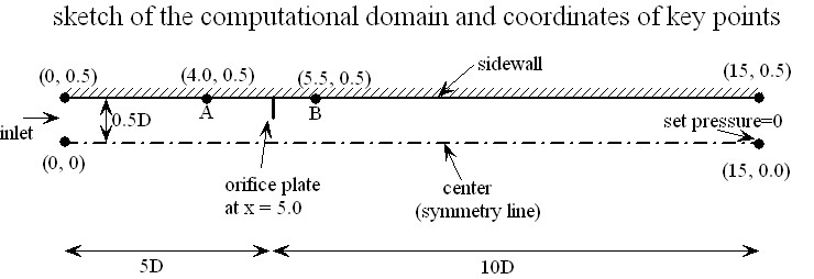
4. The domain to be used is from 5D upstream the orifice plate to 10D downstream the orifice plate.
5. Flow symmetry is observed by considering only the top half of the pipe.
Flow Reynolds number is: Re = r X D X (Q/A) / m =
800 x 1 x (0.05/0.25/ p /D2) / 1 = 51
Physical units: Pressure in Pa (N/m2) and Velocity in m/s.
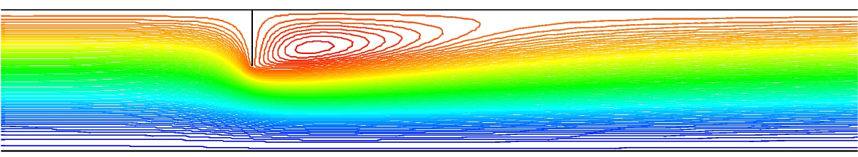
Streamlines near the orifice
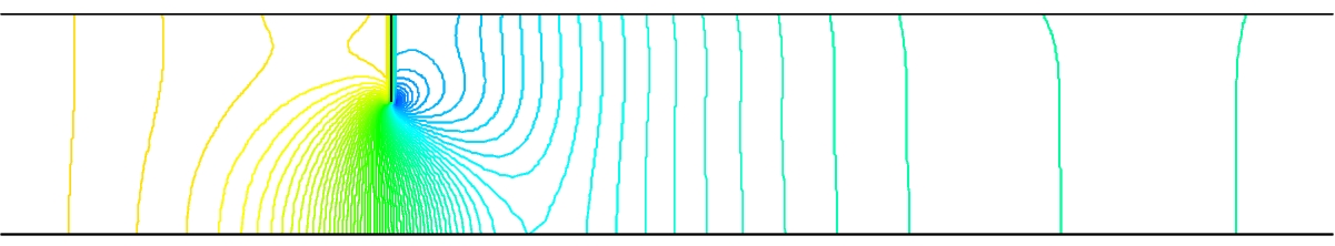
Pressure distribution near the orifice with contour interval = 2 Pa
Study:
- How does the flow change with d/D and Reynolds number?
- How does the orifice augment the pressure drop? And why?
- What factors need to be considered if the orifice plate is to be used as a practical flow-rate measurement device?
Modeling procedure and details:
- Geometry and mesh modeling using Gambit. Gambit journal file.
- Start Fluent (Start...All Programs....Fluent Inc. Products...FLUENT6.0 or FLUENT 6.1.22...FLUENT 6.1.22), select "2d" solver.
- Import mesh generated by Gambit: FILE-READ-CASE and input a mesh model. The mesh model files can be downloaded here: model0.msh, model1.msh, model2.msh, model3.msh. You MUST save these files AND the file inlet_z_velocity.c to your own directory (which you can create temporarily on "Desktop" or under "My Documents") before running your Fluent session. These files are also available under the directory "Y:\meeg102_LP_Wang".
- Check the grid: GRID-CHECK.
- Select a solver formulation: DEFINE-MODEL-SOLVER and check "Axisymmetric" under Space.
- Choose the basic equations to be solved: DEFINE-MODEL-Viscous Model and Check "Laminar".
- Set exit reference pressure to zero for convenience: DEFINE-Operating Conditions and set Operating Pressure to zero at X=15m.
- Specify material properties: DEFINE - Materials... - Set name to "myfluid", density to 800 kg/m3 and viscosity to 1 kg/m-s, Click Change/Create to replace the default "air". Click Close.
- Specify boundary conditions:
-- Interpret the source code inlet_z_velocity.c: DEFINE-User Defined - Functions- Interpreted UDFs, then type inlet_z_velocity.c in the "Source File Name" field, Click "Interpret". Then Click "Close".
-- Set the inlet boundary condition: DEFINE-Boundary Conditions -> Set "Zone=inlet" and "Type=velocity-inlet" -> Click "Set" -> replace "constant" in the last field by "udf inlet_z_velocity" for velocity magnitude normal to boundary. -> Click "OK" -> Click "Close"
-- Check other boundary conditions (in this case the default settings are OK).- Initialize the flow field: SOLVE-Initialize-Initialize, set "Compute From" field to "inlet", click "init" and then close the window.
- Adjust the solution monitor parameters:
-- SOLVE-Monitors-Residual Monitors, change the convergence Criterion for x-velocity and y-velocity to 0.0001 for better accuracy, also check "Plot" but uncheck "Print" under "Options" (top-left corner on the same panel) to allow the relative error to be plotted -> Click "OK"- Calculate the flow by iterations: Solve-Iterate, set number of iterations to 300, then click iterate. Observe how the relative errors change with the iteration number.
- Click "iterate" again for more iterations. You may stop the iterations as long as the relative errors for both velocities are below 0.0001.
- Save case and data: FILE - WRITE -Case&Data. You should save your case and data if you want to examine the solution later.
- Examine the results: See Post-processing details below.
Post-processing details:
- How to find pressure at any given location?
-- First define a point by SURFACE-POINT, then specify the location by x and y coordinates and give a name under New Surface Name. For example, the coordinates for point A and point B are (4.0,0.5) and (5.5, 0.5), respectively. You should provide a label under "New Surface Name" for each (eg, point-a, point-b).
-- Then use PLOT-XY PLOT, select "write to File", select Pressure/Static Pressure for Y-axis Function, select "point-a" from the "Surfaces" list
-- Click Write to save the pressure data for "point-a", give a name for the file
-- Open the file to obtain the pressure value.- How to plot pressure distributions from different models on a same plot?
-- Use PLOT-XY PLOT to write data to files first
-- Then use PLOT-File to load all files and replot (could first edit the label in the saved files)
-- You may modify legend and plot symbols- How to do contour plots?
-- Pressure contour: Use DISPLAY-CONTOURS, select Pressure/Static Pressure, set Levels = 100, make sure that "Color" is checked on the Page Setup menu of the graphics window.
-- Streamlines: Use DISPLAY-CONTOURS, select Velocity/Stream Function.- How to plot axial velocity profile at any axial location?
-- First define a line with two end points by SURFACE-Line/Rake, check the Line tool, enter the coordinates for two end points and give a label (say, line-4.0). For example, the line at x=4.0 can have two end-points (x=4.0, y=0.0) and (x=4.0,y=0.5). You can refer to the domain sketch above to further details.
-- Then use PLOT-XY PLOT to plot or write to a file. Make sure that you select the line label under "Surfaces" and check the "Plot Direction". The Y-Axis Function needs to be defined as "Velocity - Axial Velocity".
-- Note that you can plot axial velocity profiles at several locations in a same plot if you select all the lines you defined before you click "Plot".
-- You could define the y-axis of the plot to be the radial location by unchecking "Position on X Axis" and check "Position on Y axis".
-- You may also change the line style of the curves by clicking "Curves" and modify.- How to save a copy of the graphics window?
-- Right Click the mouse and select "Copy to Clipboard"
-- Then paste the picture to your Word document.
Other helpful notes for your lab assignment:
- The mesh model files can be downloaded here: model0.msh, model1.msh, model2.msh, model3.msh. You MUST copy these files to your own temporary directory before running your Fluent session. These files are also available under the directory "Y:\MEEG102_LP_Wang".
- Very important: The folder and files you generate on the computer will be removed everytime the system reboots, so you need to back up the files (e.g., via SSH File Transfer, email to yourself, or copy to your own portable memory device).
- Any question? Contact Ms. Stephanie Merkler in 221 Spencer Lab. She has office hours between 4:00PM to 5:00PM on Tuesday and Thursday during the weeks of April 3 to April 27. She may also be reached by email at smerkler@udel.edu.
- The lab assignment can be downloaded here
- The schedules for the eCALC labs (046 Colburn and 140 Dupont) can be found at www.engr.udel.edu/eCALC-I and www.engr.udel.edu/eCALC-II. Problems with the eCALC labs can be directed to Mr. Randy Oswald, dolphio@udel.edu, 044 Colburn Lab, (302) 831-0835.
- You may want to check back here as additional notes may be posted to address any questions and concerns that arise.