In this session we solve an unsteady flow and heat transfer in a mixing elbow using Gambit and FIDAP. Note that the geometry dimensions are given in inches, while other properties are in SI units.
 

Geometry and parameters:

The long-time (steady-state) velocoty field

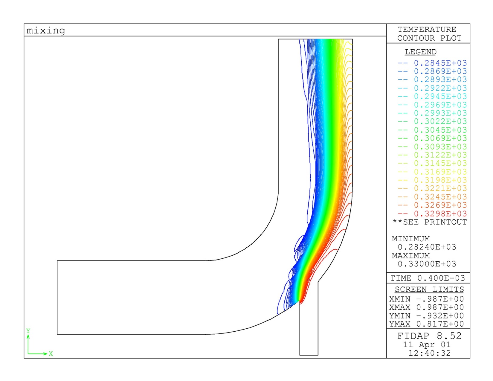
The long-time (steady-state) temperature distribution for laminar flow.

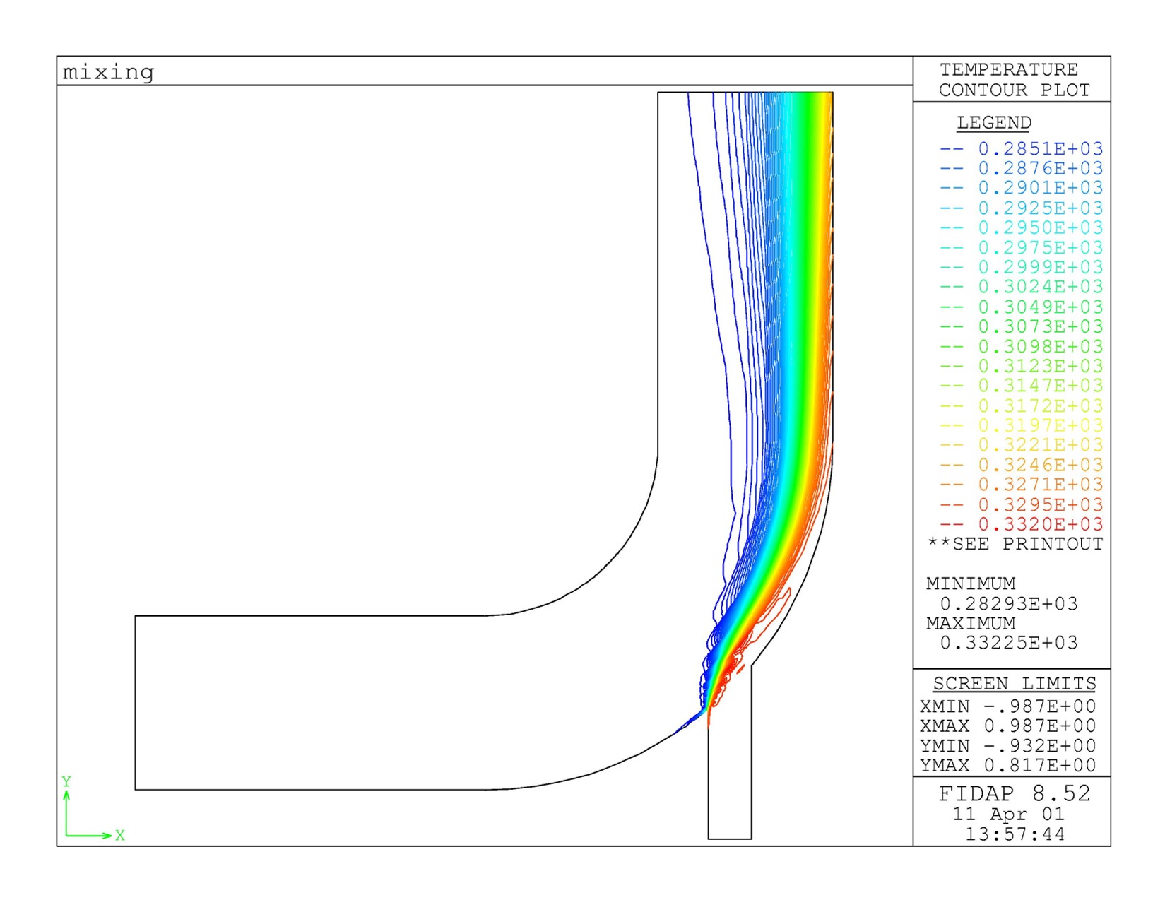
The steady-state temperature distribution for turbulent flow.

Temperature at the center of the outlet at a function of time (laminar flow).

General Instructions for Setting up the model of mixing elbow

gambit -id mixing -dev X -new

1. Select a solver
   Solver - FIDAP

2. Display 4x4 grid covering -32 < x < 32, -32 < y < 32 using
   Tools - Coordinate System - Display Grid
   
3. Pick 9 vertices 
   (-32, -32) (0.,-32) (-32,-16) (0,-16)
   (0., 0. ) (16, 0.)  (32, 0.)
   (16, 32) ( 32,32)
   using Crtl + right click

4. Remove grid by deselecting Visibility

5. Create Arcs for the bend of the mixing elbow
   Geometry - Edge - Create Edge - Arc 
   Shift + left click at point (0., 0.)     !define the center
   Left click End-Points field
   Shift + left click at points (16,0.) (0, -16)   !define end points
   Apply

   Repeat to create the outer arc.

6. Creat straight edges
    Geometry - Edge - Create Edge - Straight
    Shift + left click to select points, then apply

7. Create the small pipe for the mixing elbow

   Geometry - Edge - Split/Merge Edges
   Select the large arc
   Type = Cylindrical
   local t = -39.93
   Apply

   Select the larger portion of the nearly created arc
   local t = -50.07
   Apply

   Geometry - Vertex - Move/Copy Vertices
       ! Make a copy of nearly created vertex by shifting in y by -12
   Click Fit-to-Window

   Create another vertex by copying and shifting in x by 4

   Create the edges

8. Create faces from egdes
   
   Geometry - Face - Create Face
   Shift + left click each edge of teh large pipe, in turn, to form
    a continuous loop
   Apply 
 
   Repeat for the small pipe

9. Specify node distribution
   On Inlet and Outlet of te large pipe:
    Mesh - Edge - Mesg Egdes
    Select inlet and outlet
    Grading = Apply,  Type = Successive Ratio
    Ratio = 1.25
    Double Sided is on
    Use 10 interval counts
    Apply
  4 straight edges of the large pipes
    use 15 equal intervals 
  Large arcs:
    6 equal intervals for the center part
    12 graded intervals, ratio =0.9
     (make sure arrow pointing towards the small pipe, 
        Use shift-middle click to change direction)
  Inner arc:
    double sided, ratio = 0.85
    Turn off Option / Mesh       !Let gambit decide the mesh later
    Apply

10. Create structured mesh:
    Mesh-Face-Mesh Faces
    Select the large pipe
    Elements = Quad
    Type = Map

11. Mesh the small pipe:
    Select the small pipe
    Elements = Quad
    Type = Map
    Spacing  = 1
    Apply

12. Set Boundary Types
    Specify model Display Attributes - Mesh = off - Apply

    Zones - Specify boundary types
    name = inflow1, type = plot, Entity/Edges (select large pipe inlet), Apply
    name = outflow, type = plot, Entity/Edges (select large pipe outlet), Apply
    name = inflow2, type = plot, Entity/Edges (select small pipe inlet), Apply
    name = walls, type = plot, Entity/Edges (select all wall edges), apply
   
13. Export neutral file

   Export - Mesh - Accept

14. Exit - Save
    This will generate:
      *.jou: a journal file
      *.trn: a summary file
      *.FDNEUT: a neutral file
      *.FIPREP: FIPREP file

15. Start fidap: fidap -id mixing -gui -new
    Read mixing.FIPREP
    
16. Set up boundary and initial conditions according to the following:

/
FIPREP
 PROB (2-D, INCO, TRAN, LAMI, NONL, NEWT, MOME, ENER, FIXE, NOST, NORE, SING)
 EXEC (NEWJ)
 SOLU (S.S. = 20, VELC = 0.100000000000E-02, RESC = 0.100000000000E-02,
       ACCF = 0. )
/
 TIME (BACK, NSTE = 400, TSTA = 0. , DT = 0.1, TEND=800., VARI, WIND, NOFI, DTMA = 2.0)
 DATA (CONT)
/ Define a second coordinate system centered at large pipe inlet, Mesh Data - Coordinate
 COOR (SYST = 2, CART)
  -0.3200000000E+02, -0.2400000000E+02,  0.0000000000E+00
 PRIN (NONE)
/ Save the results every 4 steps
 POST (NBLO = 1, NOPT, NOPA)
   4, 400, 4
/ convert inch to m by SCAL, Mesh Data - Scale
 SCAL (VALU = 0.254000000000E-01)
 ENTI (NAME = "fluid", FLUI)
 ENTI (NAME = "inflow1", PLOT)
 ENTI (NAME = "inflow2", PLOT)
 ENTI (NAME = "outflow", PLOT)
 ENTI (NAME = "walls", PLOT)
 DENS (SET = 1, CONS = 1.18)
 VISC (SET = 1, CONS = 0.184000000000E-04)
 SPEC (SET = 1, CONS = 1005.0)
 COND (SET = 1, CONS = 0.260000000000E-01)
 BCNO (UX, ENTI = "inflow2", ZERO)
 BCNO (UY, ENTI = "inflow2", CONS = 0.100000000000E-01, EXCL)
 BCNO (TEMP, ENTI = "inflow2", CONS = 330.0, EXCL)
 BCNO (UX, ENTI = "inflow1", POLY = 1, SYST = 2, CART)
   0.1000000000E-01, -0.1562500000E-03,  0.0000000000E+00,  0.2000000000E+01,
   0.0000000000E+00
 BCNO (UY, ENTI = "inflow1", ZERO)
 BCNO (TEMP, ENTI = "inflow1", CONS = 283.0)
 BCNO (VELO, ENTI = "walls", ZERO, X, Y, Z)
/ The walls are adiabatic by default
 ICNO (VELO, ZERO, ENTI = "fluid", X, Y, Z)
 ICNO (TEMP, CONS = 283.0, ENTI = "fluid")
END

17. Run and postprocessing

You can use Utility/Timestep to select the time step for displaying the results.

Plot / History can be used to plot time-evolution results at any node.

FIPREP
 PROB (2-D, INCO, STEA, TURB, NONL, NEWT, MOME, ENER, FIXE, NOST, NORE, SING)
 PRES (PENA = 0.100000000000E-07, DISC)
 EXEC (NEWJ)
 SOLU (S.S. = 100, VELC = 0.100000000000E-02, RESC = 0.100000000000E-02,
       ACCF = 0.4)
 DATA (CONT)
 OPTIONS(UPWINDING)
 UPWINDING
 1 1 0 0 2 0 1 1
 PRIN (NONE)
 SCAL (VALU = 0.254000000000E-01)
 ENTI (NAME = "fluid", FLUI)
 ENTI (NAME = "inflow1", PLOT)
 ENTI (NAME = "inflow2", PLOT)
 ENTI (NAME = "outflow", PLOT)
/
 ENTI (NAME = "walls", WALL)
/ Here the ENTITY Type = WALL is very important, so that the walls will be treated with special wall elements
/ in the turbulence modeling
/
 TURBCONSTANTS
 0 0 0 0 0 0 0.9
/  Turbulent Prandtl number = 0.9, Other model constants are set to default
 DENS (SET = 1, CONS = 1.18)
 VISC (SET = 1, CONS = 0.184000000000E-04, TWO-)
 SPEC (SET = 1, CONS = 1005.0)
 COND (SET = 1, CONS = 0.260000000000E-01)
 BCNO (UX, ENTI = "inflow2", ZERO)
 BCNO (UY, ENTI = "inflow2", CONS = 10.0, EXCL)
 BCNO (TEMP, ENTI = "inflow2", CONS = 330.0, EXCL)
/ k.e. = 0.035 u^2  , diss = 0.01 u^3/D
/
 BCNO (KINE, ENTI = "inflow2", CONS = 3.5)
 BCNO (DISS, ENTI = "inflow2", CONS = 98.4)
/
 BCNO (UY, ENTI = "inflow1", ZERO)
 BCNO (UX, ENTI = "inflow1", CONS = 10.0, EXCL)
 BCNO (TEMP, ENTI = "inflow1", CONS = 283.0)
 BCNO (KINE, ENTI = "inflow1", CONS = 3.5)
 BCNO (DISS, ENTI = "inflow1", CONS = 24.6)
/
 BCNO (VELO, ENTI = "walls", ZERO, X, Y, Z)
 ICNO (VELO, ZERO, ENTI = "fluid", X, Y, Z)
 ICNO (TEMP, CONS = 283.0, ENTI = "fluid")
 ICNO (KINE, CONS = 3.5, ENTI = "fluid")
 ICNO (DISS, CONS = 24.6, ENTI = "fluid")
END