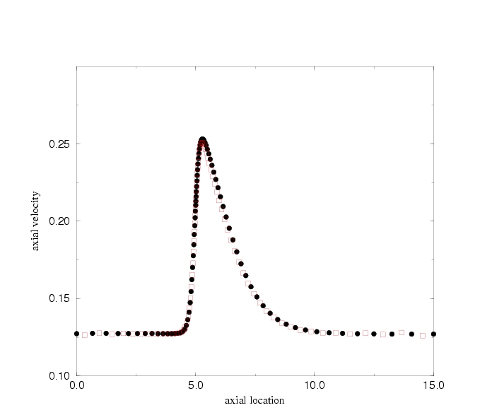
Axial velocity distribution along the centerline for d/D = 0.6: Filled circles represent FIDAP solution, squares are FLUENT solution.
Outline and Objectives:
What is FLUENT?
FLUENT is a state-of-the-art computer program for modeling fluid flow and heat transfer in complex geometries, distributed by Fluent Inc.
Contains an integrated set of components and program modules that allow fluid flow analysis
Written in C
Based on the finite volume method
General steps in using FLUENT:
FLUENT Capabilities:
Class of problems:
- 2D planar, 2D axisymmetric, 2D axisymmetric with swirl (rotationally symmetric), and 3D flows
- Steady-state or transient flows
- Incompressible or compressible flows, including all speed regimes (low subsonic, transonic, supersonic, and hypersonic flows)
- Inviscid, laminar, and turbulent flows
- Newtonian or non-Newtonian flows
- Heat transfer, including forced, natural, and mixed convection, conjugate (solid/fluid) heat transfer, and radiation
- Chemical species mixing and reaction, including homogeneous and heterogeneous combustion models and surface deposition/reaction models
- Free surface and multiphase models for gas-liquid, gas-solid, and liquid-solid flows
- Lagrangian trajectory calculation for dispersed phase (particles/droplets/bubbles), including coupling with continuous phase
- Phase change model for melting/solidification applications
- Porous media with non-isotropic permeability, inertial resistance, solid heat conduction, and porous-face pressure jump conditions
- Dynamic mesh model for modeling domains with moving and deforming mesh
- ...........
See FLUENT webpage for further details.
Modeling procedure and details:
- Geometry and mesh modeling using Gambit. Gambit journal file.
- Start Fluent, select 2d solver.
- Import mesh generated by Gambit: FILE-READ-CASE and select a mesh model.
- Check the grid: GRID-CHECK.
- Select a solver formulation: DEFINE-MODEL-SOLVER and check "Axisymmetric" under Space.
- Choose the basic equations to be solved: DEFINE-MODEL-Viscous Model and Check "Laminar".
- Set exit reference pressure to zero for convenience: DEFINE-Operating Conditions and set Operating Pressure to zero at X=15m.
- Specify material properties: DEFINE - Material properties - Set name to "orifice", density to 800 kg/m3 and viscosity to 1 kg/m-s, replace the default "air".
- Specify boundary conditions:
-- First introduce a user-defined parabolic function by the code inlet_z_velocity.c
-- Interpret the source code: DEFINE-User Defined - Functions- Interpreted UDFs
-- Set the inlet boundary condition: DEFINE-Boundary Conditions-Zone=inlet-Set and use "udf inlet_z_velocity" for velocity magnitude normal to boundary.
-- Check other bounday conditions (in this case the default settings are OK).- Initialize the flow field: SOLVE-Initialize-Initialize, set "Compute From" field to "inlet", click "init" and then close the window.
- Adjust the solution monitor parameters:
-- Solution-Monitors-Residual Monitors, change the convergence Criterion to 0.0001 for better accuracy, also check Plot to allow the relative error to be plotted.- Calculate the flow by iterations: Solve-Iterate, set number of iterations to 300, then click iterate. Observe how the relative errors change with the iteration number.
- Click "iterate" again for more iterations. You may stop the iterations as long as the relative errors for both velocities are below 0.0001.
- Save case and data: FILE - WRITE -Case&Data. You should save your case and data if you want to examine the solution later.
- Examine the results: See Post-processing details below.
Post-processing details:
- How to find pressure at any given location?
-- First define a point by SURFACE-POINT, then specify the location by x and y coordinates and give a name under New Surface Name (eg, point-a)
-- Then use PLOT-XY PLOT, select "write to File", select Pressure/Static Pressure for Y-axis Function, select "point-a" from the "Surfaces" list
-- Click Write to save the pressure data for "point-a", give a name for the file
-- Open the file to obtain the pressure value.- How to plot pressure distributions from different models on a same plot?
-- Use PLOT-XY PLOT to write data to files first
-- Then use PLOT-File to load all files and replot
-- You may modify legend and plot symbols- How to do contour plots?
-- Pressure contour: Use DISPLAY-CONTOURS, select Pressure/Static Pressure, set Levels = 100, make sure that "Color" is checked on the Page Setup menu of the graphics window.
-- Streamlines: Use DISPLAY-CONTOURS, select Velocity/Stream Function.- How to plot axial velocity profile at any axial location?
-- First define a line with two end points by SURFACE-Line/Rake, check the line tool, enter the two end points coordinates and give a name (say, line-4.0)
-- Then use PLOT-XY PLOT to plot or write to a file
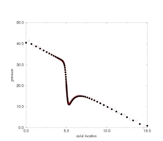
Comparing FIDAP results with FLUENT results:
| Diameter Ratio | FIDAP Result | FLUENT RESULT | Analytical |
| No orifice | 3.043 | 3.038 | 3.056 |
| d/D = 0.8 | 4.797 | 4.527 | - |
| d/D = 0.6 | 21.365 | 20.735 | - |
| d/D = 0.4 | 141.794 | 146.437 | - |
Axial velocity distribution along the centerline for d/D = 0.6: Filled circles represent FIDAP solution, squares are FLUENT solution.