• More about FIDAP

 
• Using GAMBIT to set up the same model

 
• Alternative method: ANSYS

     FIDAP: FIGEN + FIPREP  --->  2Dbed.FIJOUR

     GAMBIT: --> 2Dbed.jou, 2Dbed.trn, 2Dbed.FDNEUT, 2Dbed.FIPREP

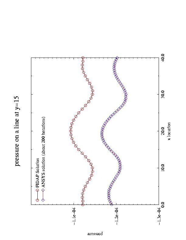
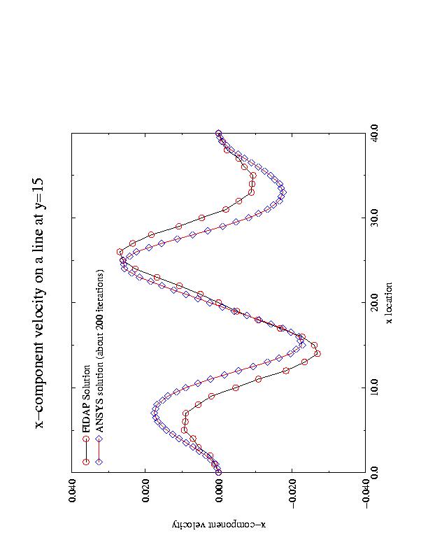
     ANSYS:  -->   2Dbed.log

More about FIDAP

This work session illustrates some advanced features of using FIDAP preprocessing and postprocessing that will let you be more productive in your FIDAP session.
 

(A) Restarting FIDAP session from previous database:
           fidap -id 2Dbed -gui -old

 (make sure that there is no file named ``id.FDIDEN''. Otherwise you will get a fatal error
message.  Always remove the file ``id.FDIDEN'' before you restart from database of a previous sesssion).

(B) Important files to save after a FIDAP session:
 

          The journal file:   id.FDJOUR  (This file contains a record of all the FIDAP commands
          executed during a previous session.)

           You should re-name the file:
           mv 2Dbed.FDJOUR 2Dbed.FDREAD

           You can simply edit the 2Dbed.FDREAD file to modify system parameters
               (such as injection velocity,   viscosity, etc.)
               (I usually only save FI-GEN and FI-PREP parts.)

           You can also define a variable to be used later on. For example,
                 $VIN=0.5
                  BCNODE(ADD, UY, ENTI = "bottom1", CONS = $VIN, X, Y, Z)

              is identical to:

                  BCNODE(ADD, UY, ENTI = "bottom1", CONS = 0.5, X, Y, Z)
 

(C) Restarting FIDAP session from a modified FDREAD file:

            fidap -id 2Dbed -gui -new

            click READFILE, input the READFILE name

            Click ACCEPT will implement all the commands in the FDREAD file
 

(D) Other files created in a FIDAP session:

FDBASE:    This is the FIDAP model database file. This is the database associated with the current problem identifier.

FDPOST: This is the results database file created by the FIDAP solver module FISOLV. This file must be made available for FIPOST to create any plots. By default, it is the FDPOST file associated with the current problem identifier.

FISTAT:   This is the FIDAP status file. All error messages are logged to this file as well as brief summary messages relating to problem setup, CPU times, memory requirements, etc.

 FIOUT :    This is the FIDAP print output file. Detailed information relating to the execution of the various commands is output to this file.

FIECHO: This is the FIDAP input echo file. This file contains an exact record of the commands input by the user.

FIPLOT:     This is the plot file created by FIPOST when the HPGL or POSTSCRIPT driver is used.

(E) On-line documentations:

You can find all on-line manuals by clicking Help,  and point the question mark on the command window you are working on.  A text window will appear which contains explanations and examples of the command and related options.

Mapped vs paved meshing:

Mapped meshing: regular checkerboard meshing.  For surface area it is limited to four-sided regions while for SOLIDs it is limited to six-sided regions.

Paved meshing: a technique for generating an automatical, well-formed
 quadrilateral mesh in arbitrary geometries.

Mesh Faces:
 

2D topological entities properly defined on which FI-GEN can produce
two-dimensional finite elements (quadrilaterals or triangles)

A mesh face consists of:

The type of meshing to be performed (mapped or paved)

One or more mesh loops that defined the boundaries of the region to be meshed

A surface that describes the geometrical variations of the region to be
meshed and on which all the nodes will lie.

A specification of the type of elements to be generated (element type and order)

Mesh Solids:
 

3D topological entities defining a volume on which FI-GEN can produce
three-dimensional finite elements (bricks or wedges)

A mesh solid consists of:

The type of meshing to be performed (mapped or plastered)

One or more mesh shells that defined the boundaries of the region to be meshed (A mesh shell is a collection of mesh faces)

A specification of the type of elements to be generated (element type: brick, wedge, or
 tetrahedron; and order: 8 or 27 node brick?)

 Mesh Generation Steps:

1. Create geometry

define points (POINT)
define curves (CURVE)
define surface (SURFACE)

2. Create mesh loops (MLOOP)

3. Create mesh faces (MFACE)

4. Create mesh shells (3D model only) (MSHELL)

5. Create mesh solids (3D model only) (MSOLID)

6. Define mesh egdes (MEDGE)

7. Generate mesh on mesh edges, mesh faces and/or mesh solid (MESH option of MEDGE, MFACE or MSOLID)

Some of the above steps may be combined.  For example, ADD by wireframe option on the MFACE
automatically generates the required surfaces, mesh loops, mesh faces, mesh shell and mesh solid directly
from a set of curves.
 

(G) Graphical View Options

You can use the View Manu to rotate, translate, and zoom in the graphics.  Or you can use  single letter commands combined with dragging the left mouse buttom to perform the same task:

``GX'' for rotation along x-axis

 ``GY'' for rotation along y-axis

``GZ'' for rotation along z-axis

``1'' for translation in x-direction

``2'' for translation in y-direction

``3'' for translation in z-direction

``T'' for translation in xy-plane

``P'' for zooming in or out

``C'' for zooming in selected region

``E'' for translating a selected point

``M'' for magnifying about a selected point  (press M, click a point in the graphics,
press a magnification number (1 through 9, 9 for maximum magnification)

``U'' for reducing about a selected point (press U, click a point in the graphics, then press a number (1 through 9)

``V'' to restore the previous view

``D'' to redraw the graphics

``F'' to fill the graphics to the entire window

``H'' to produce a hard copy

(H) Checking the database before running the solver:
 

For a big problem, do

FIPREP-Simulation-EXECUTION MODE=DATACHECK
RUN-FISOLV

to make sure you do not get any errors in the FDSTAT file.

(I) FIPOST Capabilities

FIPOST is a command-driven program which is directed to perform various task by entering commands. These commands fall into a number of different categories based on their function. Following is a partial list of important FIPOST commands grouped according to their function.

Plot Commands

Each of the Plot commands results in the display of a particular type of plot.

CONTOUR:  generalized contour plot command for contouring both solution fields and derived variables, including turbulent dissipation, turbulent kinetic energy, pressure, stream function, temperature and vorticity amongst many others

CONVERGENCE: plot convergence history of the simulation

EDGE: edge plot of model (optional display of initial and/or boundary conditions)

HISTORY:  time history plot of solution and derived variables

LINE:  plot of any solution or derived variable along any line in space

MESH: element mesh plot

PARTICLE: define particle injection points for PATH command

PATH: particle path and dye trace plot

SEARCH:  graphically query values of solution or derived values

STEP: time history plot of time increment in a transient analysis

VECTOR:  vector plot of a solution variable, including velocity, vorticity and stress

XYPLOT :  user defined x-y coordinate plot

Computation commands result in the computation and printout, as well as optional plotting, of various quantities derived from the solution variables.

COEFFICIENT:  compute heat or mass transfer coefficient at any element boundary

FLOWRATE: compute flow rate across any element boundary

FLUX:  compute heat fluxes across any element boundary

MEAN: compute the mean of a solution quantity

PROPERTY:  compute nodal property values

STRSPRINT:  compute stresses at any element boundary

YPLUS: compute turbulent y+ values at any element wall boundary

Display Commands
 

Display commands manipulate the graphics image to be displayed on the plot.

DISPLAY :  select the view direction and angle for display of an image

GCPOINT:  define the graphics control point

GROUP:  restrict plotting to selected element groups

PLANE: specify a cutting plane and active display surface for 3-D plots

RESET: reset all viewport, window and display parameters to their default values

SETWINDOW: set windows to which subsequent commands apply

TRANSFORM: compute a new variable for plotting by applying a transformation to a specified solution or derived variable

VIEWPORT:  select the area of the graphics device to be used to display the plot

WINDOW: controls all operations relating to the creation and modification of graphics windows in FIDAP

ZOOM: select the portion of the model to be displayed on the screen (using dimensionless screen units)
 

Graphics Options commands enable or disable various optional features
available for the plot commands.

AXES:   enable or disable plotting of axes on plots

BOUNDARY:  select type of boundary to be drawn surrounding the model

COLOR :  enable or disable color plotting

GRID:  select background mesh plotting on contour plots

HEADING:  select type of titling information to be displayed

PATTERN:  specify options for use of color on vector and contour plots

SETCOLOR: set or modify color tables

SUPERIMPOSE:  enable or disable superimposing of plots

XYSET: set options for x-y coordinate plots

Utility commands perform various miscellaneous functions.

DEVICE : select the device driver for graphics output

ECHO: control amount of information echoed to the screen

NEUTRAL: output solution data to a neutral file

OPTIONS: set various program options

PRINT : print out solution variables

SCALE: scale solution variables

TIMESTEP: select a time step from the results database file

TITLE:  enter new titling information for plots
 

A simple plot:

PLOT-Line-Degree of Freedom=shear-Line definition: Entity="right"-Accept

TITLE-SET PLOT TITLE-shear rate along vertical wall-ACCEPT

Utility-XYSET-Y axis minium=0-Y axis maximum=0.06-ACCEPT

Utility-Neutral-FILE FORMAT=FIPOST-Degree of Freedom=Shear-FILE name="shear.out"-ACCEPT

GRAPHICS-SETCOLOR-SETCOLOR OPTION=EDITOR, GENERAL COLOR=3, BACKGROUND=2 (white), ETC ........ (Make sure to open new window for the new color map to take effect (use Graphics-Window-Open)

EDGE-PLOTTED INFORMATION=BCNODE-NODAL D.O.F.=Velocity-ADD-Accept

Multiple display windows (display four plots simultaneously):   Example

WINDOW-WINDOW ACTION=4SPLIT

SETWINDOW-DELETE-ALL
(All window will be inactive.)

SETWINDOW-ADD-WINDOW=2
(only window 2 will be active.  See FIDAP command history window for such information.)

EDGE-PLOTTED INFORMATION=BCNODE-NODAL D.O.F.=Velocity-ADD-Accept

SETWINDOW-ADD-WINDOW=3
(only window 3 will be active. )

MESH-ACCEPT

SETWINDOW-ADD-WINDOW=4
(only window 4 will be active. )

VECTOR-PLOT TYPE=VELOCITY-ACCEPT

SETWINDOW-ADD-WINDOW=5
(only window 5 will be active. )

CONTOUR-DEGREE OF FREEDOM=Streamline-CONTOUR LEVELS: AUTOMATIC=40-ACCEPT

(K) Color Display Problem

You may experience graphic display problem if the colormap on your host does not match what FIDAP uses as default.  FIDAP uses 256 colormap.  Therefore, make sure that, on your PC, you check the DISPLAY-SETTINGS.  Change to 256 colors if necessary.  You will have to restart Exceed and FIDAP
after you change your host display settings.
 

Using GAMBIT to set up the same model

What is Gambit?

A software package by Fluent Inc. for creating geometry and mesh

Top-down approach is possible

gambit -id 2Dbed -new &

1. Select a solver
   Solver - FIDAP

2. Create 4 corner vertices
   FIT-to-Window

3. Generate boundary lines:
   Note shift + left mouse button to pick a point

4.  Use Split option to split the bottom line into 3.
    enter the coordinates for the dividing points

5. Face
   simply select all lines
   Set label = fluid

6. Mesh edge
   select all lines with spacing = 1

7. Mesh
   select the face and use mapped mesh

8. Define boundary entities:
   Zones - Specify boundary types 
   solidwall + inlet + outlet
   type = PLOT

9. Export neutral file

   Export - Mesh - Accept

10. Exit - Save
    This will generate:
      *.jou: a journal file
      *.trn: a summary file
      *.FDNEUT: a neutral file
      *.FIPREP: FIPREP file
     
11. modify *.FIPREP file:
    density
    viscosity
    boundary conditions
    
12. fidap -id 2Dbed -gui -new
    READ in *.FIPREP

13  Create date base and Run the simulation

14. Post processing

Alternative method: ANSYS

1. Set Preferences for GUI filtering to FLOTRAN CFD

2. Element type:
   Preprocessor - Element type - Add/Edit/Delete 
       - Add - Flotran CFD: 2D FLOTRAN 141
       - OK - Close

3. Geometry:

   Preprocessor - Create - Rectangle - By dimensions -
         X1=0, X2=15, Y1=0, Y2=80
   Apply

   X1=25, X2=40, Y1=0, Y2=80
   OK

   Preprocessor - Create - Areas / Arbitrary - Through KPs
   Pick points (15,0), (25,0) (25,80) (15,80)
   OK

   (Comments: This procedure will not generate multiple lines at the same location.)

4. Establish Mesh Pattern:

   Preprocessor - MeshTool - Lines / Set 
   Pick the four vertical lines, NDIV = 80
   APPLY

   Pick 4 horizantal lines near the vertical walls
   OK - NDIV = 15 - Apply
   
   Pick the 2 center horizantal lines
   OK - NDIV = 10 - OK

   Turn on Mesher Map
   MESH - Pick all 

5. Boundary Conditions:
   Preprocessor - loads - Apply - Velocity - On lines
   Pick 4 wall lines
   OK - Vx=0, Vy=0 - Apply 
 
   Pick inlet
   OK - Vx=0, Vy=0.4 - Apply
     
   Preprocessor - loads - Apply - Pressure DOF - On lines
   Pick outlet -  PRES=0. - OK

6. Fluid Properties:
   Solution - FLOTRAN Set up - Fluid Properties
   OK - Density = 0.0012, Viscosity = 1.81e-4 -
   OK
   
7. Set execution control

   Solution - FLOTRAN Set up - Execution control
   Global iterations = 40
   OK

8. Run FLOTRAN

9. Read results
   General Postproc - Read results / Last set
   
10. Plot vector field
   General Postproc - Plot results - Vector / Predefined - OK


11. Plot y-velocity on a line:
   Generate Postproc - Path operations - Define Path 
   - By nodes - pick the two node points (39,0) and (39,80)
   - name = vyplot, NDIV = 80
   - close

   Generate Postproc - Path operations - Map onto path 
   - Label=vyplot, DOF solution / VY
   OK
 
   - plot path item - on graph
   - choose vyplot
   OK
   
   - list path item
   - choose vyplot
   OK