Outline and Objectives:
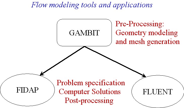
What is FIDAP?
FIDAP is a CFD (Computational Fluid Dynamics) software package distributed by Fluent Inc. (used to be Fluid Dynamics International).
Contains an integrated set of components and program modules that allow fluid dynamics analysis
Based on the finite element method
FIDAP Structure
FIDAP Capabilities:
Class of problems:
- flow of viscous fluids (compressible, incompressible)
- isothermal or non-isothermal
- laminar or turbulent flows
- single-phase or two-phase flows
- Newtonian, non-Newtonian or visco-elastic fluids
- mass transport
- ...........
See FIDAP webpage for further details.
What is Gambit?
A software package by Fluent Inc. for creating geometry and high-quality mesh
Both bottom-up and top-down approach are possible
Easy to use
Allow CAD/CAE integration
......
For further details, see GAMBIT Webpage.
The most efficient way to learn software packages is that people
show you how to solve a simple
problem using the software....
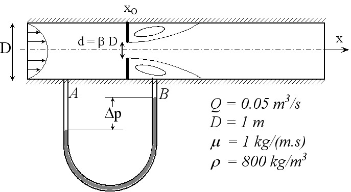
Example: Flow modeling in a pipe with an concentric orifice plate
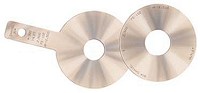
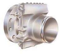
Orifice plates and fitting
1. Pipe diameter D = 1 m, fluid viscosity m = 1 kg/(m.s), density r = 800 kg/m3.
2. Orifice diameter d = 0.6D
3. Total in-coming flow rate Q = 0.05 m3/s
4. The domain to be used is from 5D upstreaming the orifice plate to 10D downstream the orifice plate.
5. Flow symmetry is observed by considering only the top half of the pipe.
Flow Reynolds number is:
Re = r X D X (Q/A) / m =
800 x 1 x (0.05/0.25/ p /D2) / 1 = 51
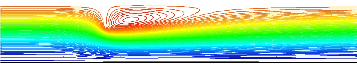
Streamlines
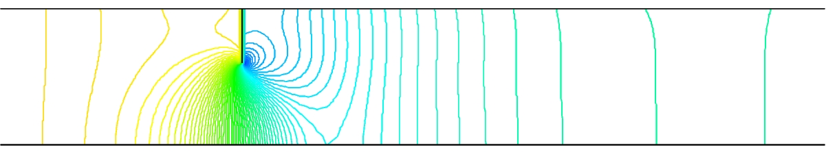
Pressure distribution with contour interval = 2 Pa
Study:
- How does the flow change with Reynolds number and d/D?
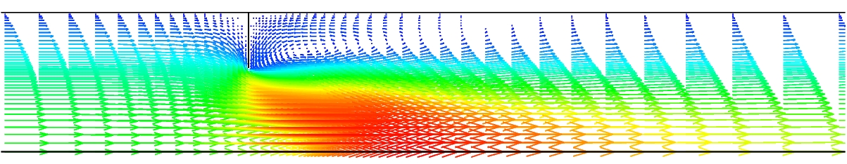
- How does the velocity distribution change through the orifice?
- How does the orifice augment the pressure drop?
The Step-by-Step Instructions - Gambit preprocessing and FIDAP simulation modeling
1. gambit -id ofepipe -new &

1a. Select a solver
     Solver - FIDAP

2. Create 9 vertices at
   X Y    Z
   0 0    0
   0 0.5  0
   0 0.3  0
   5 0.5  0
   5 0.3  0
   5 0.0  0
   15 0.0 0
   15 0.3 0
   15 0.5 0

   Geometry Command - Vertex Command - Local x,y,z - Apply

   Note Mouse Controls of the graphics:
   Left click to rotate
   Middle click to translate
   Right click to zoom in and out

3. Generate all boundary lines:
    Geometry Command - Edge Command  - Create Edge - Select Points - Apply
    Note shift + left mouse button to pick a point or points

4. Create four rectanglar faces
   Geometry Command - Face Command  - Form Face - Select Edges - Apply

6. Mesh edges with non-uniform intervals
   Mesh Command - Edge Command
   Three short vertical lines next to wall:  Double sided 1.1, 20 intervals
   Three short vertical lines next to center:  invert ratio 1.1, 20 intervals
   Horizontal edges before the orifice:   invert ratio 1.15, 30 intervals
   Horizontal edges after the orifice:   ratio 1.10, 50 intervals

   You may zoom in to check the mesh points on edges and adjust as necessary

7. Mesh the faces
   Mesh Command - Face Command
   select all the faces and use mapped mesh

8. Define Fluid and boundary entities:
   Zones Command - Specify Continuum Types Command
   Select all faces to be continuum "fluid" Entity

   Zones Command - Specify boundary types
   sidewall, orifice,  inlet, outlet,  center
   type = PLOT

9. Export mesh neutral file

   Export - Mesh - Accept

10. Exit - Save
    This will generate:
      ofepipe.jou: a journal file
      ofepipe.trn: a summary file
      ofepipe.FDNEUT: a neutral file
      ofepipe.FIPREP: FIPREP file

11. Start FIDAP:

    fidap -id ofepipe -gui -new

12. Import the gambit mesh into FIDAP
     - FICONV - ACCEPT
     - Click inputfile
     - Set FILE = "ofepipe.FDNEUT"
     - Click Accept
     - Click "END" to exit FICONV

13.  Run FIPREP

     - Click FIPREP

13A. Defining entity labels

    - Select ``Entity''
    - Left click the question mark to select ``fluid'' entity for NAME
    - Input ``Fluid'' in the ENTITY TYPE field, Right click ADD - ADD (REPEAT)
    - Left click the question mark to select ``inlet'' entity
    - Input ``plot'' in the ENTITY TYPE field, Right click ADD - ADD (REPEAT)
    - Repeat this for the other boundary entities:
         ``outlet'', ``sidewall'',``orifice'',``center''.
    - Close the "Entity Command" window by clicking "Cancel"

13B. Specifying fluid properties

     - Click Properties
     - double Click ``DENSITY''
     - Input 800.0 in the MODEL TYPE-CONSTANT field
     - Click ADD
     - double Click ``VISCOSITY''
     - Input 1.0 in the MODEL TYPE-CONSTANT field
     - Click ADD

13C. Specifying the problem type

     - Select Simulation
     - Click EXECUTION
     - Change EXECUTION MODE to NEWJOB
     - Click ADD
     - Click PROBLEM
     - Change Geometry Type to AXI-SYMMETRIC
     - Change CONVECTIVE TERM to NONLINEAR
     - Click ADD
     - Click SOLUTION
     - Change S.S. = 100, Solution Tolerance = 0.0001, Residual Tolerance = 0.0001
     - Click ADD

13D. Specifying boundary conditions

     - Click Boundary C.
     - Click BCNODE
     - Right-click exclamation point next to DEGREE of FREEDON
     - Pick VELOCITY
     - Right-click exclamation point next to REGION SELECTION
     - Pick ENTITY
     - Left-click question mark beside REGION SELECTION field
     - Pick ``sidewall''
     - Right-click exclamation point next to VALUE GENERATION field
     - Pick Zero
     - Right-select ADD(REPEAT)
     - Do the same for ``orifice''
     - Right-click exclamation point next to DEGREE of FREEDON
     - Pick URC
     - Left-click question mark beside REGION SELECTION field
     - Pick ``inlet''
     - Right-click exclamation point next to VALUE GENERATION field
     - Pick Zero
     - Right-select ADD(REPEAT)
     - Right-click exclamation point next to DEGREE of FREEDON
     - Pick UZC
     - Left-click question mark beside REGION SELECTION field
     - Pick ``inlet''
     - Right-click exclamation point next to VALUE GENERATION field
     - Pick POLYNOMIAL, set value =  1
     - Right-select ADD(REPEAT)
     - In the INPUT field, type:
       0.127324, -0.509296, 0, 2, 0
        (meaning UZC = 0.127324 -0.509296 X^0 Y^2 Z^0)
     - Right-click exclamation point next to DEGREE of FREEDON
     - Pick URC
     - Left-click question mark beside REGION SELECTION field
     - Pick ``center''
     - Right-click exclamation point next to VALUE GENERATION field
     - Pick Zero
     - Right-select ADD

     - Click END to exit FIPREP

NOTE: Step 12, 13A-13D together will generate the following ofepipe.FIJOUR file:

FICONV( NEUT, INPU, RESU, DATA )
INPUTFILE( FILE = "ofepipe.FDNEUT" )
END(  )
FIPREP(  )
ENTITY( ADD, NAME = "fluid", FLUI )
ENTITY( ADD, NAME = "inlet", PLOT )
ENTITY( ADD, NAME = "outlet", PLOT )
ENTITY( ADD, NAME = "sidewall", PLOT )
ENTITY( ADD, NAME = "orifice", PLOT )
ENTITY( ADD, NAME = "center", PLOT )
DENSITY( ADD, SET = 1, CONS = 800 )
VISCOSITY( ADD, SET = 1, CONS = 1 )
EXECUTION( ADD, NEWJ )
PROBLEM( ADD, AXI-, INCO, STEA, LAMI, NONL, NEWT, MOME, ISOT, FIXE, NOST, NORE,
SING )
SOLUTION( ADD, S.S. = 100, VELC = 0.0001, RESC = 0.0001, ACCF = 0 )

BCNODE( ADD, VELO, ENTI = "sidewall", ZERO, X, Y, Z )
BCNODE( ADD, VELO, ENTI = "orifice", ZERO, X, Y, Z )
BCNODE( ADD, URC, ENTI = "inlet", ZERO, X, Y, Z )
BCNODE( ADD, UZC, ENTI = "inlet", POLY = 1, SYST = 1, CART )
0.127324, -0.509296,     0,     2,     0
BCNODE( ADD, URC, ENTI = "center", ZERO )
END(  )

Alternatively, you may modify the ofepipe.FIPREP from the GAMBIT run to look like:
/          CONVERSION OF NEUTRAL FILE TO FIDAP Database
/
FICONV( NEUTRAL )
INPUT( FILE="ofepipe.FDNEUT" )
OUTPUT( DELETE )
END
/
TITLE
ofepipe
/
FIPREP(  )
$Umean = 0.063662
$vis = 1.0
$dens = 800.0
$umax=2.0*$Umean
$CC = -8.0*$Umean
/
ENTITY( ADD, NAME = "fluid", FLUI )
ENTITY( ADD, NAME = "sidewall", PLOT )
ENTITY( ADD, NAME = "orifice", ATTACH="fluid", PLOT )
ENTITY( ADD, NAME = "inlet", PLOT )
ENTITY( ADD, NAME = "outlet", PLOT )
ENTITY( ADD, NAME = "center", PLOT )
/
DATAPRINT( ADD, CONT )
PROBLEM( ADD, AXI-, INCO, LAMINAR, NONL, ISOTHERMAL )
SOLUTION( ADD, S.S. = 100, VELC = 0.0001, RESC = 0.0001, ACCF = 0 )
PRINTOUT( ADD, ALL, BOUN )
EXECUTION( ADD, NEWJ )
/
BCNODE( ADD, VELO, ENTI = "sidewall", ZERO )
BCNODE( ADD, VELO, ENTI = "orifice", ZERO )
BCNODE( ADD, UZC, ENTI = "inlet", POLY = 1)
    $umax,    $CC,     0,     2,     0
BCNODE( ADD, URC, ENTI = "inlet", ZERO )
BCNODE( ADD, URC, ENTI = "center", ZERO )
DENSITY( ADD, SET = 1, CONS = $dens )
VISCOSITY( ADD, SET = 1, CONS = $vis )
END(  )
/

14. Create the database

    a. Click CREATE
    b. Select Create
    c. Click ACCEPT

15. Solving the problem

    a. Click RUN
    b. Pick FISOLV
    c. Pick FOREGROUND
    d. Click ACCEPT (Now relax and wait for the simulation to finish,
        this may take a minute or two)

16. Link to the solution data base for post-processing
    a. Click IDENT
    b. Click ACCEPT

17. Start FIPOST (the post-processing module)

    a. Click FIPOST
    b. Click ACCEPT

17A. Visualizing the vector velocity field

    - Click Vector
    - Click Accept

17B. Zoom in
     - Click Graphics
     - Click Windows
     - Click ZOOM
     - Set: XMIN = -0.45, XMAX = -0.05, YMIN = -0.2, YMAX = 0.2
     - Click Accept

17C. Plotting streamlines

    - Click Contour
    - Right-click exclamation point next to DEGREE of FREEDON
    - Pick STREAMLINE
    - Input 80 in the CONTOUR LEVELS-AUTOMATIC field
      (this will draw 80 countour levels in stead of 10 by default).
    - Click ACCEPT (You can clearly see the recirculation region)

17D. Draw boundary lines
    - Click Display
    - Click Boundary
    - Set Boundary Option to POINTS = 8
    - In the INPUT field, type
       0.,0.5,0.,1    / note the last 1 meaning "pen down"
       5.,0.5,0.,1
       5.,0.3,0.,1
       5.,0.5,0.,1
       15.,0.5,0.,1
       15.,0.0,0.,1
       0.,0.0,0.,1
       0.,0.5,0.,2     / note the last 2 meaning "pen up"

17E. Line plot
     - Click PLOT
     - Click Line
     - Set DEGREE OF FREEDOM = PRESSURE
     - Set Line Definition = 2POINTS
     - Accept
     - INPUT: 0.,0.,0.,15.,0.,0.

17F. Superimpose plots
     SUPERIMPOSE( ON )
     /
     $y1 = -0.05
     $y2 = 0.30
     /
     / Use A for symbols
     / Note symbol list: 1=O, 2=+, 3=*, 4=X, 5=o, 6-31=A-Z, 32-41=0-9
     / "EVERY" for every data point
     / It is important to set the same Max and Min values.
     /
     XYSET( YMAX = $y2, Ymin = $y1, EVERY=6)
     LINE( UZC, 2POI )
         4,     0,     0,     4,   0.5,     0
     / Use B for symbols
     XYSET( YMAX = $y2, Ymin = $y1, EVERY=7)
     LINE( UZC, 2POI )
      5,     0,     0,     5,   0.5,     0
     / Use C for symbols
     XYSET( YMAX = $y2, Ymin = $y1, EVERY=8)
     LINE( UZC, 2POI )
      5.5,     0,     0,   5.5,   0.5,     0
     SUPERIMPOSE( OFF )
Print a hard copy of FIPOST visualizations
    - Click Graphics
    - Click Device
    - Select Postscript as Device driver, then Accept
    - Run FIPOST (all the plots are now saved in a file ofepipe.ps)
How to print out the value of a variable at given points?
For example, to print out pressure at two points:

FIPOST: Utility - Print:
Degree of Freedom = Pressure, Region definition = Point, Point file = "ppoints.dat"
The "ppoints.dat" may look like:
4
4.0,0.5,0.
5.5,0.5,0.
4.0,0.0,0.
5.5,0.0,0.
(Note the first line is the number of points, second and third lines are
the x,y,z coordinates for these points. You may specify any number of
points in the file.)
Also check results in ofepipe.FIOUT as needed.
Summary
     GAMBIT: --> ofepipe.jou, ofepipe.trn, ofepipe.FDNEUT, ofepipe.FIPREP
     Modify ofepipe.FIPREP
     FIDAP: FICONV, FIPREP, CREATE, RUN FISOLV, IDENT, FIPOST
            --> ofepipe.FIJOUR, ofepipe.FIOUT, ofepipe.ps etc.
     Save and modify ofepipe.FIJOUR if needed.