Objectives:
 

• Introduction to FIDAP

 
• FIDAP preprocessing: Mesh setup

 
• Example: 2D viscous flow in a channel bed

What is FIDAP?

FIDAP is a CFD (Computational Fluid Dynamics) software package distributed by Fluent Inc. (used to be Fluid Dynamics International).

Contains an integrated set of components and program modules that allow fluid dynamics analysis

Based on the finite element method
 

FIDAP Structure
 

• FI-GEN: Mesh generation module

 
• FIPREP:  Problem data specification
•  type of problems and equations, solution procedure,
•  fluid / material properties,
•  initial and boundary conditions

• FISOLV: Computational simulations

 
• FIPOST: Post processor module

FIDAP Capabilities:
 

Class of problems:
 

• flow of viscous fluids (compressible, incompressible)
• isothermal or non-isothermal
• laminar or turbulent flows
• single-phase or two-phase flows
• Newtonian, non-Newtonian or visco-elastic fluids
• mass transport
• ...........

The most efficient way to learn a software  is that people show you how to solve a simple
problem using the software....

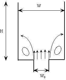
Example: steady viscous flow in a channel bed

1. Channel dimension: 40 cm by 80 cm (W=40 cm, H=80cm);

2. Central opening (W₀) at the bottom is 10cm wide, with injection velocity of 0.4 cm/s

3. Fluid (air) viscosity n= 1.81x10 ^{- 4} g/cm.s;  Fluid density r = 0.0012 g/cm³
 

Define superficial velocity u₀ = mass flux /cross-sectional area:

 u₀ = 0.4 cm/s x 10 cm  / 40  cm  =  0.10 cm/s

Flow Reynolds number is:

Re =   r u₀ W / n = 0.0012 x 0.10 x 40 / 1.81x10 ^{- 4}  =  26.5
 
 

• How does the flow pattern change with u₀ (or Re number) for given injection width?

 
• How does the flow pattern change with the opening width W₀ for a given u₀?

 
• What is the pressure change during this flow expansion?

The Step-by-Step Instruction

This is a step-by-step instruction to set up and solve the channel bed problem using FIDAP.
 
 

 Starting the FIDAP GUI:
 

          1. telnet mahler.udel.edu or strauss.udel.edu

          2. login with your username and passward

          3. cd /tmp

          4. mkdir lwang (make a new directory)

          5. cd lwang (Always start in a new, empty directory)

          6. fidap    -id    2Dbed    -gui    -new   &   (start a FIDAP session named 2Dbed)

          7. click the ``FIDAP version window'' to remove it

Setting up the flow model:
 

Start up FI-GEN (the mesh generation module):

 1. Click FI-GEN

 2. Click Accept  (after a few seconds a graphical window appears)

Generating the Geometry (i.e., Points, Curves and Surfaces):

 1. Click Point

 2. Select Add under COMMAND OPTION

 3. Enter the coordinates of the following eight points: (0,0),(15,0),(25,0),(40,0),(40,80),(25,80),(15,80),(0,80)
(Will be referred to as points 1 through 8 in this order)

4. Move the cursor into the graphical window and type the letter
         ``F'' to bring all the 8 points into the window
        (you should see all the 8 points, each marked by a plus sign)

5. Click Curve(1)

6. Select ADD Line under COMMAND OPTION

7. Left click the 8 points in the graphical window in order, and finally click point 1 again.

8. Right click the mouse buttom
           (you should see lines connecting the points)

9. Left click points 2 and 7, then right click
        (a vertical line is drawn)

10. Left click points 3 and 6, then right click
        (another vertical line is drawn)
 

11 . Click Mesh Face

12. Select ADD by W/F

13. Left click the 4 lines connecting the points 1-2, 2-7, 7-8, 8-1 in order, then right click (a mesh face is defined, you should see a blue cross)

14. Left click the 4 lines connecting the points 2-3, 3-6, 6-7, 7-2 in order, then right click

15. Left click the 4 lines connecting the points 3-4, 4-5, 5-6, 6-3 in order, then right click

1. Click Mesh Edge

 2. Select ADD

 3. Input 80 in the ``Interval'' box field

4. Left click the four vertical lines connecting the points 1-8,2-7,3-6,4-5;

5. Right click (you should see 80 nodes on each of the vertical line)

6. Input 15 in the ``Interval'' box field

 7. Left click the four horizontal line sections connecting the points 1-2,3-4,5-6,7-8;

 8. Right click

 9. Input 10 in the ``Interval'' box field

 10. Left click the two horizontal line sections connecting the points 2-3,6-7

 11. Right click

 12. Click Mesh Face

 13. Select Mesh

 14. Click ``All'' under SELECT OPTION

 15. Click ``Map'' under MESH FACE DEFAULTS

 16. Input ``fluid'' in the ``Entity'' box

 17. Right click in the graphical window (You should see uniform mesh drawn)

Specifying entity names for the boundaries:
 

 1. Click Mesh Edge

 2. Select MESH MAP

 3. Left click the line connecting points 1 and 8

 4. Input ``left'' in the ``Entity'' field

 5. Right click in the graphical window

 6. Left click the line connecting points 4 and 5

 7.  Input ``right'' in the ``Entity'' field

 8. Right click in the graphical window

 9. Left click the lines connecting points 5-6,6-7,7-8

 10. Input ``top'' in the ``Entity'' field

 11. Right click in the graphical window

 12. Left click the lines connecting points 1-2,3-4

 13. Input ``bottom'' in the ``Entity'' field

 14. Right click in the graphical window

 15. Left click the line connecting points 2-3

 16.  Input ``inlet'' in the ``Entity'' field

 17. Right click in the graphical window

 18. Click END once to exit FI-GEN

 Defining entity labels
 

 1. Click FIPREP, Select ``Entity''

 2. Left click the question mark to select ``fluid'' entity

 3. Input ``Fluid'' in the ENTITY TYPE field, Right click ADD - ADD (REPEAT)

 4. Left click the question mark to select ``left'' entity

 5. Input ``plot'' in the ENTITY TYPE field, Right click ADD - ADD (REPEAT)

 6. Repeat this for the other boundary entities:  ``right'', ``top'',``bottom'',``inlet''.

 Specifying fluid properties
 

 1. Click Properties

 2. double Click ``DENSITY''

 3. Input 0.0012 in the MODEL TYPE-CONSTANT field

 4. Click ADD

 5. double Click ``VISCOSITY''

 6. Input 1.81e-4 in the MODEL TYPE-CONSTANT field

 7. Click ADD
 

 1. Click Boundary C.

 2. Click BCNODE

 3. Right-click exclamation point next to DEGREE of FREEDON

 4. Pick VELOCITY

 5. Right-click exclamation point next to REGION SELECTION

 6. Pick ENTITY

 7. Left-click question mark beside REGION SELECTION field

 8. Pick ``left''

 9. Right-click exclamation point next to VALUE GENERATION field

 10. Pick Zero

 11. Right-select ADD(REPEAT)

 12. Do the same for ``right'', ``bottom'' boundaries

 13. Right-click exclamation point next to DEGREE of FREEDON

 14. Pick UX

 15. Left-click question mark beside REGION SELECTION field

 16. Pick ``inlet''

 17. Right-click exclamation point next to VALUE GENERATION field

 18. Pick Zero

 19. Right-select ADD(REPEAT)

 20. Right-click exclamation point next to DEGREE of FREEDON

 21. Pick UY

22. Left-click question mark beside REGION SELECTION field

 23. Pick ``inlet''

 24. Right-click exclamation point next to VALUE GENERATION field

25. Pick CONSTANT, and input 0.4 (meaning that the injection velocity
is 1.0 cm/s or the Reynolds number based on the superficial velocity or mass flux is (0.4/4)x 0.0012 x 40/1.81e-4 = 26.5)

 26. Right-select ADD

 Specifying the problem type
 

 1. Select Simulation
 2. Click EXECUTION
 3. Change EXECUTION MODE to NEWJOB
 4. Click ADD
 5. Click PROBLEM
 6. Change CONVECTIVE TERM to NONLINEAR
 7. Click ADD
 8. Click END to exit FIPREP

 Creating the Database
 

 1. Click CREATE
 2. Select Create
 3. Click ACCEPT

 Solving the problem
 

 1. Click RUN
 2. Pick FISOLV
 3. Pick FOREGROUND
 4. Click ACCEPT (Now relax and wait for the simulation to finish, this may take a minute or two)
 

 1. Click IDENT
 2. Click ACCEPT
 3. Click FIPOST
 4. Click ACCEPT

 Visualizing the vector velocity field
 

 1. Click Vector
 2. Click Accept

 Plotting streamlines
 

 1. Click Contour

 2. Right-click exclamation point next to DEGREE of FREEDON

 3. Pick STREAMLINE

 4. Input 80 in the CONTOUR LEVELS-AUTOMATIC field (this will draw 80 countour levels in stead of 10 by default).

 5. Click ACCEPT (You can clearly see the recirculation region)
 

 1. Click Utility

 2. Select XYSET

 3. left-click Y AXIS MINIMUM and input 0.0 as YMIN

 4.  left-click Y AXIS MAXIMUM and input 0.02 as YMAX

 5. left-click GRID LINES and right-click the exclamation point to
        select HVGRID

 6. click ACCEPT

 7. Click PLOT

 8. Select LINE

 9. Right-click exclamation point next to DEGREE of FREEDON

10. Pick SHEAR

11. Right-click  exclamation point next to LINE DEFINITION to pick
         ENTITY

12. Left-click the question mark to select ``left''

13. Click ACCEPT (this will plot the local shear rate as a function
         of height on the left boundary, at the end of recirculation, the
         shear rate reaches a minimum value of near zero.
          This happens at y=44 cm for this case.)

 Exit FIDAP (always remember to exit FIDAP properly)
 

 Click END to exit FIPOST
 Click END one more time to exit FIDAP
 Answer YES to the EXIT PROMPT question

 Print a hard copy of FIPOST visualizations
 
 

 1. Click Graphics
 2. Click Device
 3. Select Postscript as Device driver, then Accept
 4. Run FIPOST (all the plots are now saved in a file 2Dbed.FIPLOT)
 5. Exit FIDAP
 6. fdp2ps
 7. Enter 2Dbed.FIPLOT as plot file
 8. Name the postscript file as you like
 

 How to print out the value of a variable at given points?

For example, to print out pressure at two points:

FIPOST: Utility - Print: 
Degree of Freedom = Pressure, Region definition = Point, Point file = "infile"

The "infile" may look like:
2
20.,0.,0.
20.,80.,0.

(Note the first line is the number of points, second and third lines are
the x,y,z coordinates for the two points. You may specify any number of
points in the file.)