Outline and Objectives:
Important things to know about ANSYS:
      ansys -g -j jobname

      For other start-up options,
      see Chapter 3 of Operation Guide.
--------------------------------------------------------
FILE TYPE           FILE NAME          FILE FORMAT

Log file            jobname.log        ASCII

Error file          jobname.err        ASCII

Output file         jobname.out        ASCII

Database file       jobname.db         Binary

Results file:                          Binary
 Solid/Structural   jobname.rst
 Thermal            jobname.rth
 Fluid              jobname.rfl

------------------------------------------------------
The log file is the most important file. It keeps a complete log
  of an ANSYS session (list all commands you execute). You can
  read the log file, view it while in ANSYS,  edit it,
  and input it later.
  Note: use ! for comments

To input a log file: FILE - Read input from ...

The error file lists all the errors and warnings. You may use
  this to edit your log file.

Output file:
  containing:
      -- Load summary information,
      -- mass and moments of inertia of the model
      -- solution summary information
      -- total CPU time,
      -- data requested by the OUTPR output control command
          e.g., General Postprocesser - list results - modal -
           - print output
  If you run the solution interactively, the output
  file is actually your screen (window). By doing the following
  before issuing SOLVE, you can divert the output
  to a file instead of the screen:
    File - Switch Output to - File

Database file: Contains all model information

Results file: contains solution data generated during SOLVE steps
PlotCtrls - Style - Size and Shape
Plot - Elements
-- graphical display: contour, deformed shape, reaction force..

-- tabular listings (can be saved in the output file)
(1) PlotCtrls: changing graphics specifications
     Plot: select graphics action

(2) Replot and Erase:
       Plot - Replot
       PlotCtrls - Erase Options - Erase Screen

(3) Multi-Plotting Techniques
      (a) PlotCtrls - MultiWindow Layout
      (b) PlotCtrls - Multi-Plot Controls

(4) Storing a graphics display on a file:
     PlotCtrls - Redirect Plots - to Graphics File
Two-dimensional modeling of the Steel Plate using ANSYS
You can use ANSYS to answer the question:
To what extent is one-D solution adequate?
The two-D solid-element model for the Steel Plate problem:
Mesh resolution: 32x8, namely 32 elements in X and 8 elements in Y
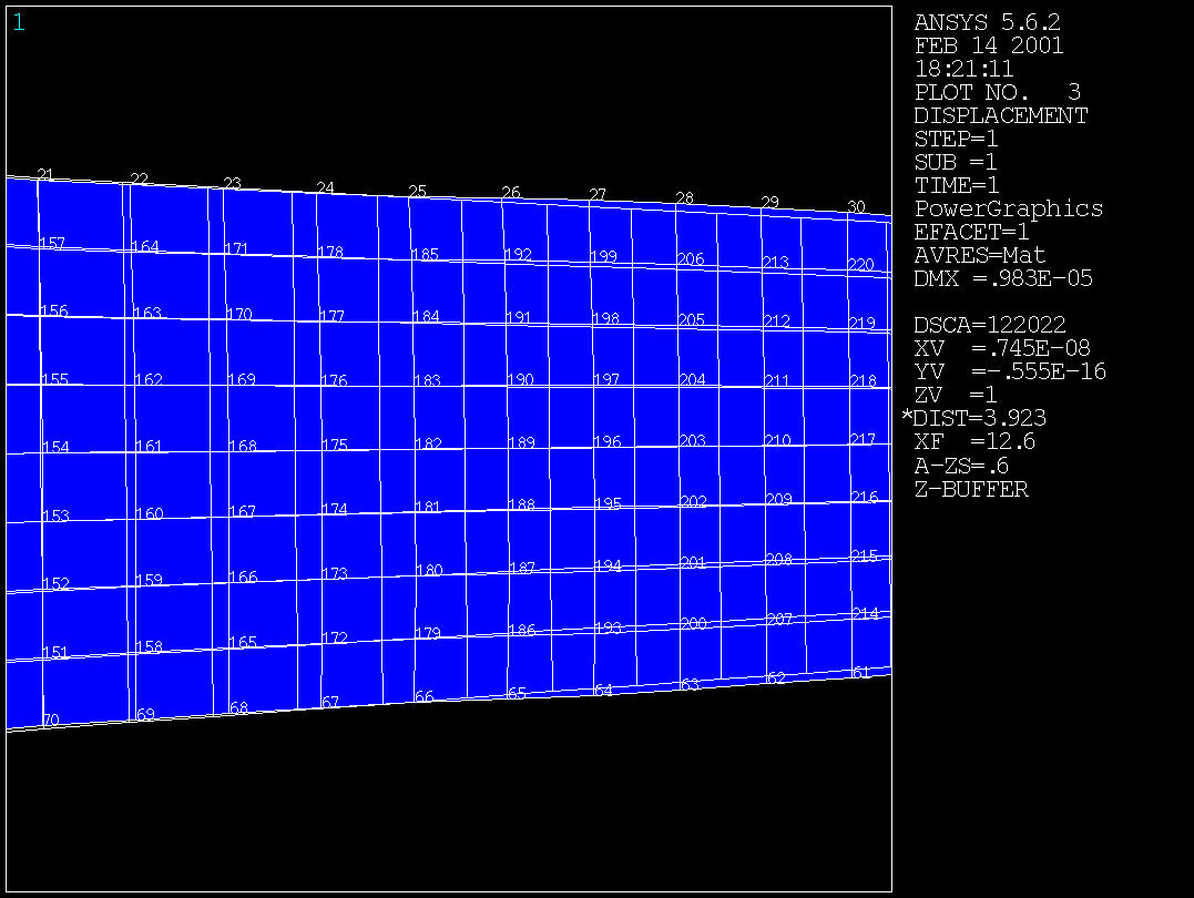
Objective: (1) Study the effect of external load distribution
(2) Study the effect of different Poisson ratio
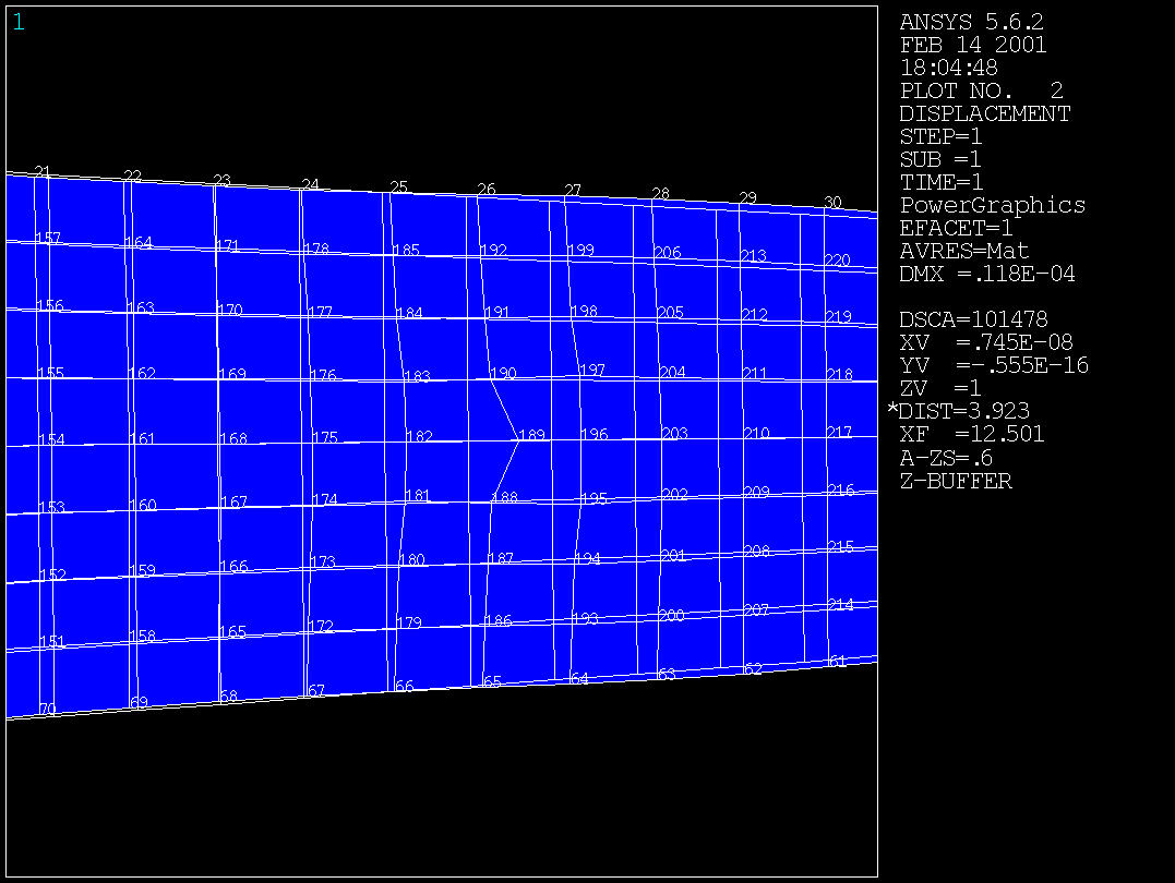
Model Development (for Poisson ratio=0.3, Load over 1/2 of width):
Here are the steps for setting up the model.
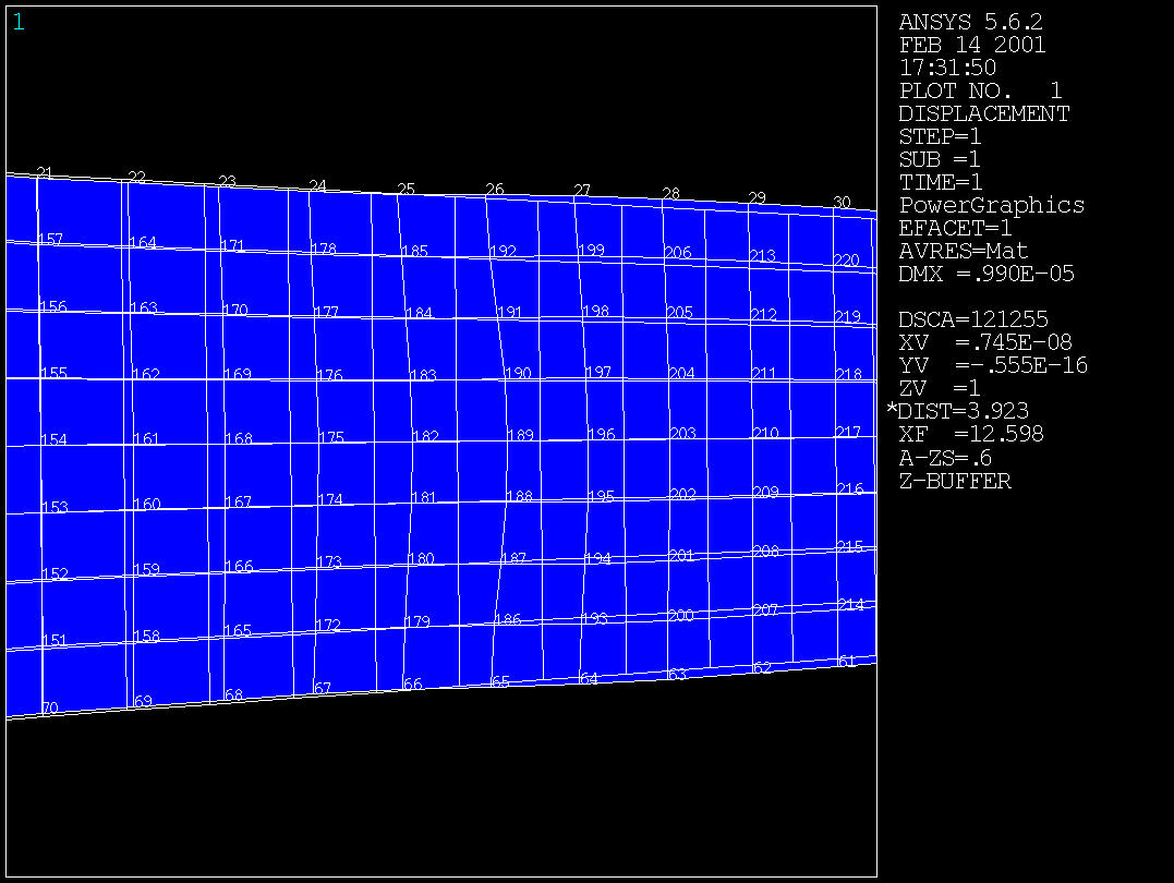
| Load distribution / Poission Ratio | Displacement at x=12 and y=0 (Node 189) | Displacement at x=24 and y=0 (Node 46) |
| 1/8 Width / 0.3 | 11.825e-6 | 9.8755e-6 |
| 1/4 Width / 0.3 | 10.601e-6 | 9.8717e-6 |
| 1/2 Width / 0.3 | 9.8965e-6 | 9.8642e-6 |
| Full Width / 0.3 | 9.2886e-6 | 9.8343e-6 |
| 1/8 Width / 0.0 | 11.488e-6 | 9.9281e-6 |
| 1/4 Width / 0.0 | 10.420e-6 | 9.9248e-6 |
| 1/2 Width / 0.0 | 9.8126e-6 | 9.9183e-6 |
| Full Width / 0.0 | 9.3139e-6 | 9.8922e-6 |
| 1D Links (2) | 9.2720e-6 | 9.9527e-6 |
| 1D analytical solution | 9.2707e-6 | 9.8684e-6 |
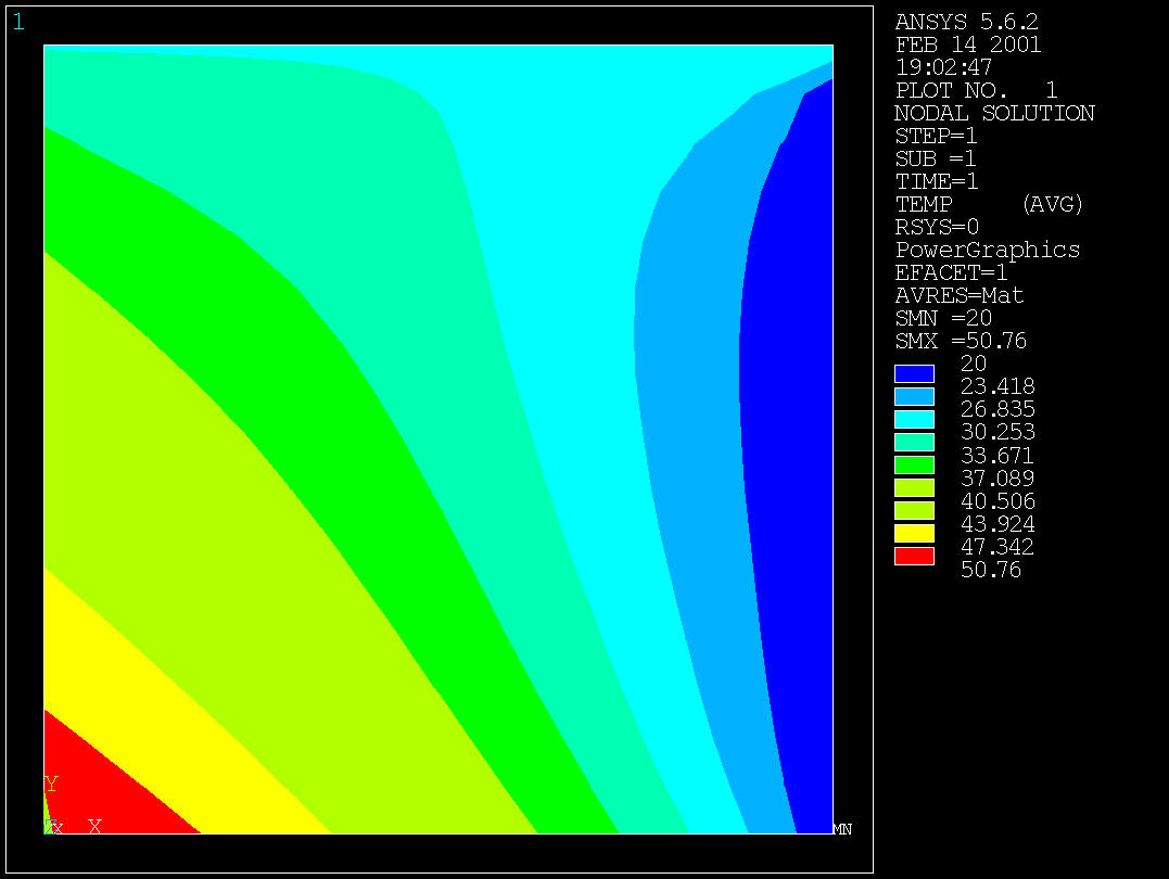
Two-dimensional modeling of heat conduction using ANSYS

Consider heat conduction in an aluminum plate (12in x 12in x 2in thick or
30.5 cm x 30.5 cm x 5.1 cm)
subject to the following boundary conditions:

  Two edges are heated using thermally bonded electrical resistance strip
   heaters (assume constant heat flux boundary condition)

  The other two edges are cooled using thermally bonded heat exchanger
   plates supplied with cooling water from a chiller
   (assume constant temperature boundary condition)

  The bottom face is insulated with glass wool

  The top face is separated from the surroundings by an air gap trapped
  underneath a glass plate

Assume: T1 = 20 C, T2=30 C, q1 = 10000 W/m^2, q2=15000 W/m^2.
Material properties: conductivity = 200 W/m.k.

Treat this as a 2D heat conduction problem. Solve for temperature
distribution.
Here are the steps for setting up the model.
 Note that you can perform a full three-D solution with ANSYS and compare
that with the 2D results.
Note that you can perform a full three-D solution with ANSYS and compare
that with the 2D results.