MEEG 342: Computer Project I
Numerical Solution of Two-Dimensional, Steady-State
Temperature
Distribution in a Rectangular Domain
Purpose
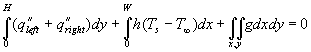
The purpose of this assignment is to apply the finite difference numerical technique to solve the steady-state heat conduction equation, given by
![]() (1)
(1)
where T is the temperature, x and y are the physical coordinates of the domain, g is the volumetric rate of internal heat generation (in W/m3 ), and k is the thermal conductivity. Note that such a heat generation would, for example, be caused by passing electric current through the material. Also note that a common mistake is not to include the heat generation rate in the proper units (recall that it represents energy per unit volume ).
Problem Definition
A two-dimensional solid (the third dimension is so long that the temperature does not vary in that direction) generates heat internally. One surfaces of the solid is insulated, two of the other surfaces are in contact with a body at constant temperatures To and T1 respectively and one surface is cooled with a coolant. We are interested in the steady state temperature distribution.
As you know, the solution of Equation (1) gives the distribution of temperature in a Cartesian domain. This expression is a second-order, linear partial differential equation. As in analytical solutions, we need to specify boundary conditions in order to solve the problem. In this assignment, we will use the mixed type of boundary conditions.
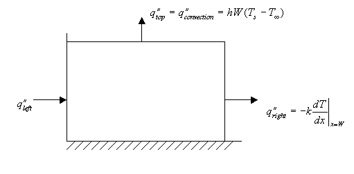
Let us consider the domain shown below in
Figure
1. The block is assumed to have a height H and a width W. A
two-dimensional analysis assumes that the domain is either infinitely
deep
(such as a long bar, with temperature independent of the z direction),
or that
it is a finite block where the two surfaces parallel to the x-y plane
are
perfectly insulated.
The boundary conditions are:
![]() at y = 0
at y = 0
![]() at y = H
at y = H
![]() at x = 0
at x = 0
![]() at x = W
at x = W
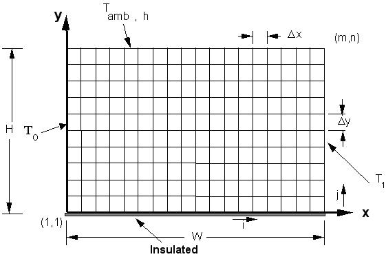
Figure 1. Problem
definition
Numerical Solution Approach
Divide the domain into (m-1) parts in the x-direction and (n-1 ) parts in the y-direction. Discretization of the domain requires m nodes by n nodes for the mesh size, requiring a dimension statement for the temperature of real T(m,n). The individual nodes are numbered (i,j), where i=1,2,3,.....m and j=1,2,3,....n, related as shown below in Figure 2.
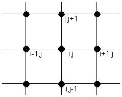
Figure 2. Grid cell
notation
In addition, we will use the following for the width, height, and boundary temperatures
W = 60 cm
H = 30 cm To=
160C T1
= 100 C Tamb = 20 C
SOLUTIONS
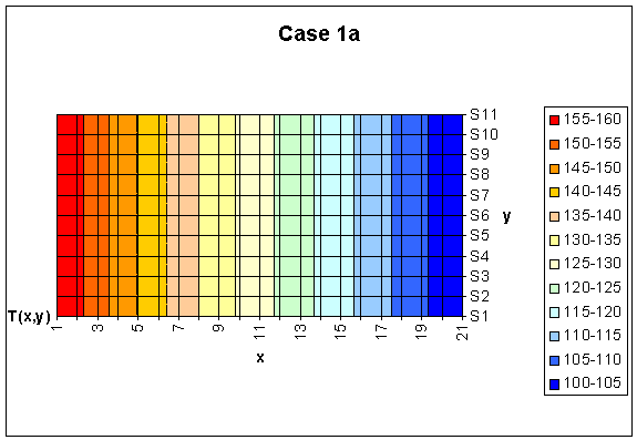
Case 1a: m=21, n=11, k=2 W/m C
, g=0,
h=0
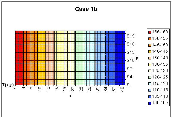
Case 1b: m=41, n=21, k=2 W/m C , g=0, h = 0
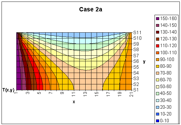
Case 2a: m=21, n=11, k=2 W/m C , g=0, h = 500 W/m2 C
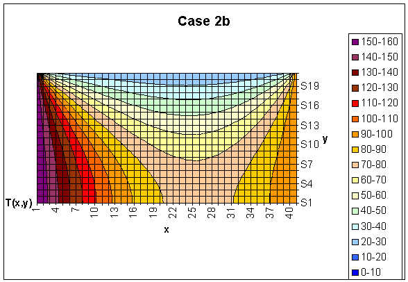
Case 2b: m=41, n=21, k=2 W/m C , g=0, h = 500 W/m2 C
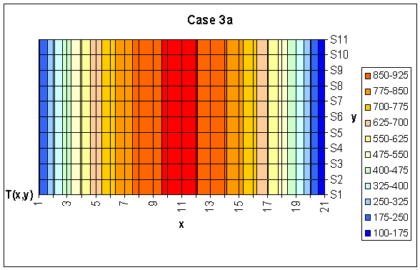
Case 3a: m=21,
n=11, k= 50
W/m C , g=0.9 MW/m3 , h=0
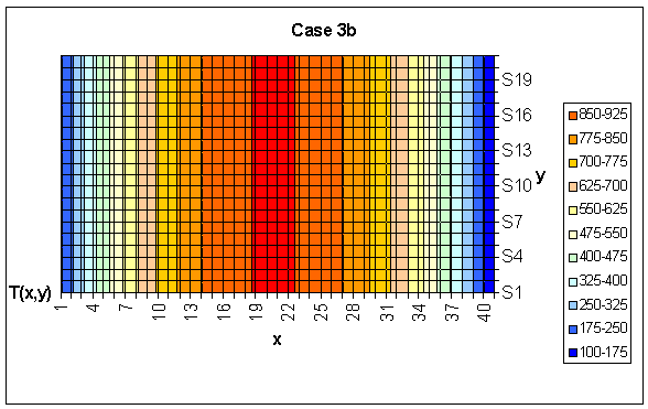
Case 3b: m=41,
n=21, k= 50
W/m C , g=0.9MW/m3 , h=0
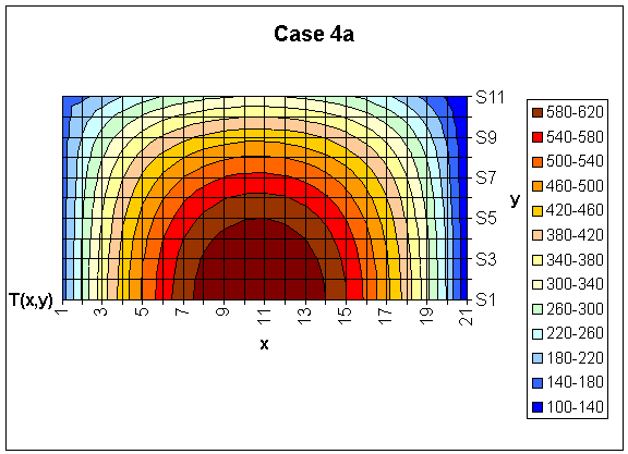
Case 4a: m=21,
n=11, k=50
W/m C , g=0.9 MW/m3, h = 500 W/m2 C
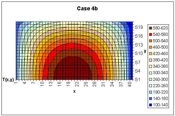
Case 4b: m=41, n=21, k=50 W/m
C ,
g=0.9 MW/m3, h = 500 W/m2 C
![]()
Since T is not a function of x and y, the partial differential equation turns to an ordinary differential equation. And with g = 0;
![]()
where a, b are
constants. From BC’s, ![]() at x = 0 and
at x = 0 and ![]() at x = W, the analytical solution is
at x = W, the analytical solution is
![]()
With numerical values
![]()
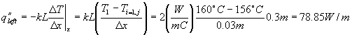
Calculate q that needs
to be supplied along the left wall to maintain the wall temperature at
T0
analytically and compare it with the calculations of q for case 1a and
1b. Repeat
the procedure at the right wall for this case. Remember for Case 1, the
q
supplied through the left wall should be leaving through the right wall
under
steady state conditions with no heat generation.
And the heat flux from left to right
![]()
![]()
With numerical values for case 1a, at the left the heat flux for unit depth is

For case 1b with the same formulas, ![]() and
and ![]()
For case b, the results are closer to the analytical solution.
The error for the left wall decreases from %31 to %26 and for the right wall, from %5 to %3.
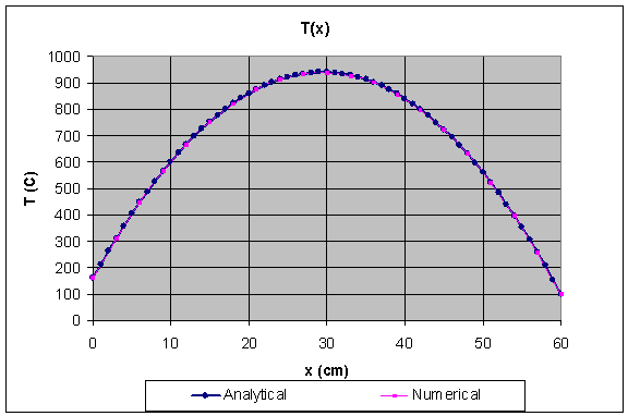
Compare the
temperature solution for case 1a and 1b with analytic solution for
the
temperature in the x-direction for steady state and no heat
generation.
Case 1a

Case 1b
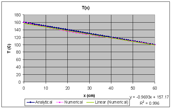
As it seen from the figures, although the numerical solution is very close to the analytical one for both cases, in the second one the accuracy is better.
The Energy balance,

![]()
![]() and g
= 0
and g
= 0
For unit depth and Fourier law at the left and the right wall,
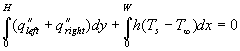
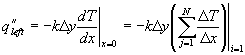
For the numerical solution, one can get the heat flux by using the sum,
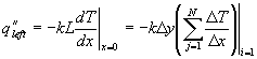
![]()
Calculate the error in
the energy balance for case 2a and 2b.
Case 2a:
![]()
Case 2b:
![]()
In the second case, better accuracy is obtained. This is simply a result of finer mesh.
Find
the analytical solution for the temperature along the x direction and
compare
it with the numerical solutions obtained for cases 3a and 3b. Also
calculate
the q along the left and right wall and compare it with the analytic
solution.
![]()
Since T is not a function of x and y, the partial differential equation turns to an ordinary differential equation. And with nonzero g term;
![]()
where b, c
are constants. From BC’s, ![]() at x = 0 and
at x = 0 and ![]() at x = W, the constants can be found.
at x = W, the constants can be found. ![]() and
and ![]() then,
then,
![]()
With numerical values
![]()
And the heat flux for unit depth
![]()
At the left and the right wall the analytical solution of heat flux is,
![]()
![]()
With numerical values for case 3a, at the left the heat flux is,
![]()
![]()
And for case 3b,
![]()
![]()
The errors are found as follows, Case
a @left, Error
= %5.2
Case a @right, Error =
%3.1
Case b @left, Error = %5.0
Case b @right, Error =
%3.0.
For case b, the error decrease from %5 to %3.
For both cases the analytical and the numerical solution are same and the temperature distribution curves fit.
By using the same method in question 4 for case 2 and this time adding the heat generation term to the energy balance,
The Energy balance,


![]()
![]()
For unit depth and Fourier law at the left and the right wall,
For the numerical solution, one can get the heat flux by using the partial sum which is actually the discretization of the integral,
![]()
![]()
Calculate the error in
the energy balance for case 4a and 4b.
Case 4a:
![]()
Case 4b:
![]()
The effect of finer mesh can be seen here from these results. In the second case, the result is closer to zero.
The accuracy of a solution in finite difference method is related with the number of meshes used in the discretization. Therefore, in cases b the accuracy is better than those of in cases a.
Convergence of a numerical solution depends on the convergence accuracy defined in the sample code. Decreasing the convergence accuracy leads to more accurate results.
The effect of thermal conductivity coefficient can be seen by comparing the first two and the last two cases. When k is increased from 2 to 50, heat transfer increases. The heat generation leads to higher temperatures and higher thermal conductivity is required in order to transfer heat from the system and avoid high temperatures that might cause melting of the material.
Extra Notes…
Derivation of the equations by using finite difference method for the top boundary:
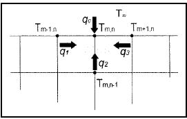
The Energy balance,
![]()
![]()
With dx=dy=![]() and for unit depth,
and for unit depth,
![]()
Since we have half of the cell,
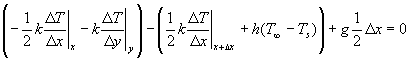
![]() in the figure above.
Divide by k all terms,
in the figure above.
Divide by k all terms,

Rearrange the equation by multiplying all terms
with ![]()
![]()
![]()
Sample Code
'MEEG302 Heat Transfer
'example program for computer assignment 1
'this program calculates the temperature distribution in a simple
'rectangular domain with constant heat flux at the top and constant
'temperature at the other three sides
Sub sample()
'define constants
Const M = 21 'grid size
Const N = 11 '
Const X = 0.6 'rectangular dimensions (m)
Const Y = 0.3 '
Const g = 900000 'heat generation
Const h = 0 'convection coefficient
Const T0 = 160 'constant temperature at side : left
Const T1 = 100 'constant temperature at side : right
Const Ts = 20 'surrounding temp
Const EPS = 0.01 'convergence accuracy
Const k = 50 'conduction coeff
'define arrays and variables
Dim Tnew(M, N), T(M, N) As Single 'temperatures
Dim isConverged As Boolean 'flag
Dim dx, dy As Single 'delta x and delta y
'initialize variables
dx = X / (M - 1)
dy = Y / (N - 1)
'initialize the temperature array
For i = 1 To M
For j = 1 To N
T(i, j) = 125
Tnew(i, j) = 125
Next j
Next i
'**** main loop
'this loop keeps recalculating the temperature field until
'it has converged
Do
'Tnew() holds the newly calculated temperatures
'T() holds the values from the last iteration
'top boundary (convection)
For i = 2 To M - 1
j = N
Tnew(i, j) = (1 / (2 * (2 + h * dx / k))) * (2 * T(i, j - 1) + T(i - 1, j) + T(i + 1, j) + 2 * h * dx * Ts / k + g * dx * dy / k)
Next i
'left boundary (constant temp)
For j = 1 To N
i = 1
Tnew(i, j) = T0
Next j
'right boundary (constant temp)
For j = 1 To N
i = M
Tnew(i, j) = T1
Next j
'bottom boundary (constant temp)
For i = 2 To M - 1
j = 1
Tnew(i, j) = (1 / 4) * (2 * T(i, j + 1) + T(i - 1, j) + T(i + 1, j) + g * dx * dy / k)
Next i
'interior nodes
For i = 2 To M - 1
For j = 2 To N - 1
Tnew(i, j) = (1 / 4) * (T(i - 1, j) + T(i + 1, j) + T(i, j - 1) + T(i, j + 1) + g * dx * dy / k)
Next j
Next i
'check to see if the temperatures have converged
isConverged = True
For i = 1 To M
For j = 1 To N
If Abs(T(i, j) - Tnew(i, j)) > EPS Then isConverged = False
Next j
Next i
'copy new temperatures to old temperatures and display on the worksheet
For i = 1 To M
For j = 1 To N
'this command displays the elements of T on the worksheet
'the command is Cells(row,column)
'because Excel counts rows from the top the grid is
'actually printed upside down
Cells(j + 1, i + 1) = Tnew(i, j)
'copy new temperatures to old array T
T(i, j) = Tnew(i, j)
Next j
Next i
'stop the loop if the values have converged
Loop While (isConverged = False)
End Sub