I:
 Þ
Þ
 Þ
Þ
 Þ
Þ
![]() Þ
Þ
![]()
At x=0, ![]() Þ c1=0
Þ c1=0
At x=1, T=200 Þ ![]()
Thus, ![]()
(a) The maximum temperature in the rod is
![]() °C (at
x=0)
°C (at
x=0)
(b) The heat loss at x=L is
![]() (W)
(W)
II:
(a) Finite difference equations at the two ends and in the interior.
Node # 1:
![]()
![]() , because at node1, it’s just half of a
cell. The g(dx/4) is the average g(x) in the half of cell of node1.
, because at node1, it’s just half of a
cell. The g(dx/4) is the average g(x) in the half of cell of node1.
![]()
![]()
Node # M:
![]() (°C)
(°C)
Interior nodes (i=2 to M-1):
![]()
Where ![]()
![]()
(b) Program (M=10) using Matlab:
heattransfer_rod.m
%numeric
solution for one dimension steady-state conduction
%MEEG342
Heat Transfer
%'program
for computer assignment 1
%'this
program calculates the temperature distribution in a rod with heat generation,
%'insulated
at one end, constant temperature at the other end, and side surfaces insulated.
function
heattransfer_rod
global M L Tend EPS dx
k A S ifConverged Q_out X i T Tanal
%---------------------define
constants--------------------------
% M is the
grid size, but the initiation of M is done in plot_curve.m
% we can
initiate the M with 30 or 10, then the final temperature result
% will be
different
L=1; %rod
length
Tend =200; %constant
temperature at one end
EPS =0.01;%convergence
accuracy
%--------define
and initial arrays ---------------------------
T=ones(1,M); %As Single 'temperatures
T=T*Tend; %Initial
the temperature array with Tend
Tnew=ones(1,M); %As the new caculated temperatures
Tnew=Tnew*Tend; %Initial
the array with Tend
Tanal=zeros(1,M); %As Single analytical solution
X=zeros(1,M); %As Single coordinate of nodes
%-----------------initial
variables---------------------------------
ifConverged=0; %As
Boolean flag,initial it as false=0
dx=L/(M-1); %As Single
%delta x
k=100; %As Single
thermal conductivity
A=100000; %As Single
coefficient of heat generation
S=25/10000; %As Single
cross sectional area of the rod
%analytical
solution
for i=1:M
X(i) =(i - 1)*dx;
Tanal(i)=
366.7-166.7*(X(i))^3;
end
%------------main
loop------------------------------------------------
%this loop
keeps recalculating the temperature field until
%it has
converged
while ifConverged==0 %continue
the loop if the values doesn't converged
%Tnew() holds the newly calculated temperatures
%T() holds the values from the last iteration
%left end
(insulated)
Tnew(1)=T(2)+A*(dx^3)/(8*k);
%right end
(constant temperature)
Tnew(M)=Tend;
%Interior
nodes
for i=2:(M - 1)
Tnew(i)=(1/2)*(T(i-1)+T(i+1))+A*(i-1)*(dx)^3/(2*k);
end
%check to
see if the temperatures have converged
ifConverged=1;
for i =1:M-1
if
abs(T(i)-Tnew(i))> EPS
ifConverged
=0;
end
end
T=Tnew;
end
%copy new
temperatures to old temperatures and display on the worksheet
T=Tnew;
%calculate
the heat loss at the right end
Q_out=A*(L - dx/4)*S*(dx/2) + k*S*(T(M - 1) - T(M)) / dx;
Plot_curve.m
%the file is to
plot the temperature distribution when M=30 and M=10
%the
global variables which is defined and used in heattransfer_rod.m
global M X T
Tanal
%set the
value of the M
M=30;
heattransfer_rod;%runing the
heattransfer_rod.m to caculate T
%plot the
Temperature when M=30
%plot the
numeric solution of Temperature vs X coordinate
figure;
plot(X,T,'--rs','LineWidth',1,...
'MarkerEdgeColor','k',...
'MarkerFaceColor','g',...
'MarkerSize',8);
hold on;
%plot the
analytic solution of T
plot(X,Tanal,'--rp','LineWidth',1,...%plot the
analytic solution of T
'MarkerEdgeColor','k',...
'MarkerFaceColor','g',...
'MarkerSize',8)
% give the graph the title
title('curve of
temperature distribution ');% give the graph the title
% give the
x coordinate a label
xlabel('x--unit(m)');
% give the
y coordinate a label
ylabel('Temperature--unit(K)');
hold all;
%plot the Temperature
when M=10
M=10;
%runing
the heattransfer_rod.m to caculate T, when M=10
heattransfer_rod;
%plot the
numeric solution of Temperature vs X coordinate
plot(X,T,'--yd','LineWidth',1,...
'MarkerEdgeColor','k',...
'MarkerFaceColor','y',...
'MarkerSize',8);
hold all;
%plot the
analytic solution of T
plot(X,Tanal,'--gp','LineWidth',1,...%plot the
analytic solution of T
'MarkerEdgeColor','k',...
'MarkerFaceColor','r',...
'MarkerSize',8);
legend('T when M=30','Tanal when
M=30','T when M=10','Tanal when
M=30',4);
(c) Plot the temperatures
M=10:
|
X(i) |
Tanal(i) |
T(i) |
|
0 |
366.6667 |
366.087 |
|
0.111111 |
366.438 |
365.9165 |
|
0.222222 |
364.8377 |
364.3763 |
|
0.333333 |
360.4938 |
360.0944 |
|
0.444444 |
352.0348 |
351.699 |
|
0.555556 |
338.0887 |
337.8181 |
|
0.666667 |
317.2839 |
317.0798 |
|
0.777778 |
288.2487 |
288.1121 |
|
0.888889 |
249.6113 |
249.5428 |
|
1 |
200 |
200 |
|
|
Q(L)= |
124.9745 |
M=30:
|
X(i) |
Tanal(i) |
T(i) |
|
0 |
366.6667 |
365.9573 |
|
0.034483 |
366.6598 |
365.9532 |
|
0.068966 |
366.612 |
365.9099 |
|
0.103448 |
366.4821 |
365.7866 |
|
0.137931 |
366.2293 |
365.5422 |
|
0.172414 |
365.8125 |
365.1357 |
|
0.206897 |
365.1906 |
364.526 |
|
0.241379 |
364.3227 |
363.6722 |
|
0.275862 |
363.1678 |
362.5331 |
|
0.310345 |
361.6849 |
361.0678 |
|
0.344828 |
359.833 |
359.2351 |
|
0.37931 |
357.571 |
356.9941 |
|
0.413793 |
354.8581 |
354.3037 |
|
0.448276 |
351.6531 |
351.1228 |
|
0.482759 |
347.915 |
347.4104 |
|
0.517241 |
343.603 |
343.1252 |
|
0.551724 |
338.6759 |
338.2265 |
|
0.586207 |
333.0928 |
332.6729 |
|
0.62069 |
326.8127 |
326.4235 |
|
0.655172 |
319.7944 |
319.4371 |
|
0.689655 |
311.9972 |
311.6727 |
|
0.724138 |
303.3799 |
303.0891 |
|
0.758621 |
293.9016 |
293.6454 |
|
0.793103 |
283.5213 |
283.3002 |
|
0.827586 |
272.1978 |
272.0127 |
|
0.862069 |
259.8904 |
259.7417 |
|
0.896552 |
246.5579 |
246.446 |
|
0.931034 |
232.1593 |
232.0845 |
|
0.965517 |
216.6537 |
216.6162 |
|
1 |
200 |
200 |
|
|
Q(L)= |
124.7409 |
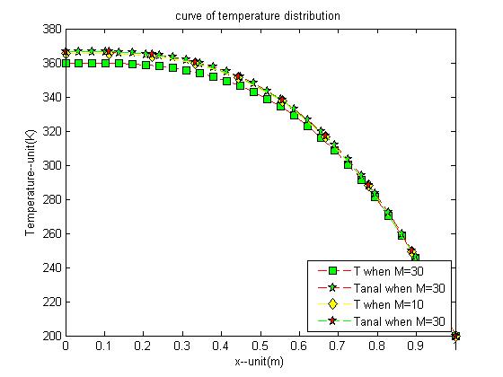
Temperature distribution
From the figure, we can see that both results (M=10 and M=30) are very close to analytic solution.
(d) Heat Loss
By running the programs, we find the heat loss at x=L is
Q = 124.9745 (W) when M = 10, and
Q = 124.7409 (W) when M = 30,
while the analytic solution is
Q = 125 (W)